

149
Large Geometry MOSFET Compact Models
φ
φ
φ
s
s
sL
c
y
y
y L
V
( ) =
=
=
0
0
at
at
and
h h
sb
sb
ds
y
V
y
V V
y L
( ) =
=
+
=
at
at
0
(4.52)
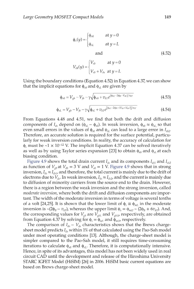
Using the boundary conditions (Equation 4.52) in Equation 4.37, we can show
that the implicit equations for f s0 and f sL are given by
φ
γ φ
φ
φ
s
g b
f b
s
kT
V
v
V V
v e
s
B
sb
kT
0
0
2
0
=
−
−
+
−
−
(
)
(4.53)
φ
γ φ
φ
φ
sL
gb
fb
sL
kT
V V
v
V V
v e
sL
B
s b
d s
k T
=
−
−
+
−
−
+
[
]
2
(
)
(4.54)
From Equations 4.48 and 4.51, we find that both the drift and diffusion
components of I ds depend on (f sL − f s0 ). In weak inversion, f s0 ≈ f sL, so that
even small errors in the values of f s0 and f sL can lead to a large error in I ds2 .
Therefore, an accurate solution is required for the surface potential, particularly for weak inversion conditions. In reality, the accuracy of calculation for
f s must be ~1 × 10 −12 V. The implicit Equation 4.37 can be solved iteratively
as well as by using Taylor series expansion [23] to obtain f s0 and f sL at each
biasing condition.
Figure 4.9 shows the total drain current I ds and its components I ds1 and I ds2
as function of V gb at V db = 3 V and V sb = 1 V. Figure 4.9 shows that in strong
inversion, I ds ≈ I ds1 , and therefore, the total current is mainly due to the drift of
electrons due to V ds . In weak inversion, I ds ≈ I ds2 , and the current is mainly due
to diffusion of minority carriers from the source end to the drain. However,
there is a region between the weak inversion and the strong inversion, called
moderate inversion, where both the drift and diffusion components are important. The width of the moderate inversion in terms of voltage is several tenths
of a volt [24,25]. It is shown that the lower limit of f s ≡ f mL in the moderate
inversion is ~(2f B − v kT ), whereas the upper limit f s = f mU ~ (2f B + 6v kT ). And,
the corresponding values for V gb are V gbL and V gbU , respectively, are obtained
from Equation 4.37 by solving for f s = f mL and f mU , respectively.
The comparison of I ds − V ds characteristics shows that the Brews chargesheet model predicts I ds within 1% of that calculated using the Pao-Sah model
under most operating conditions [13]. Although, the charge-sheet model is
simpler compared to the Pao-Sah model, it still requires time-consuming
iterations to calculate f s0 and f sL . Therefore, it is computationally intensive.
Hence, in spite of its advantages, this model has not been widely used in real
circuit CAD until the development and release of the Hiroshima University
STARC IGFET Model (HiSIM) [26] in 2006. HiSIM basic current equations are
based on Brews charge-sheet model.
Large Geometry MOSFET Compact Models
φ
φ
φ
s
s
sL
c
y
y
y L
V
( ) =
=
=
0
0
at
at
and
h h
sb
sb
ds
y
V
y
V V
y L
( ) =
=
+
=
at
at
0
(4.52)
Using the boundary conditions (Equation 4.52) in Equation 4.37, we can show
that the implicit equations for f s0 and f sL are given by
φ
γ φ
φ
φ
s
g b
f b
s
kT
V
v
V V
v e
s
B
sb
kT
0
0
2
0
=
−
−
+
−
−
(
)
(4.53)
φ
γ φ
φ
φ
sL
gb
fb
sL
kT
V V
v
V V
v e
sL
B
s b
d s
k T
=
−
−
+
−
−
+
[
]
2
(
)
(4.54)
From Equations 4.48 and 4.51, we find that both the drift and diffusion
components of I ds depend on (f sL − f s0 ). In weak inversion, f s0 ≈ f sL, so that
even small errors in the values of f s0 and f sL can lead to a large error in I ds2 .
Therefore, an accurate solution is required for the surface potential, particularly for weak inversion conditions. In reality, the accuracy of calculation for
f s must be ~1 × 10 −12 V. The implicit Equation 4.37 can be solved iteratively
as well as by using Taylor series expansion [23] to obtain f s0 and f sL at each
biasing condition.
Figure 4.9 shows the total drain current I ds and its components I ds1 and I ds2
as function of V gb at V db = 3 V and V sb = 1 V. Figure 4.9 shows that in strong
inversion, I ds ≈ I ds1 , and therefore, the total current is mainly due to the drift of
electrons due to V ds . In weak inversion, I ds ≈ I ds2 , and the current is mainly due
to diffusion of minority carriers from the source end to the drain. However,
there is a region between the weak inversion and the strong inversion, called
moderate inversion, where both the drift and diffusion components are important. The width of the moderate inversion in terms of voltage is several tenths
of a volt [24,25]. It is shown that the lower limit of f s ≡ f mL in the moderate
inversion is ~(2f B − v kT ), whereas the upper limit f s = f mU ~ (2f B + 6v kT ). And,
the corresponding values for V gb are V gbL and V gbU , respectively, are obtained
from Equation 4.37 by solving for f s = f mL and f mU , respectively.
The comparison of I ds − V ds characteristics shows that the Brews chargesheet model predicts I ds within 1% of that calculated using the Pao-Sah model
under most operating conditions [13]. Although, the charge-sheet model is
simpler compared to the Pao-Sah model, it still requires time-consuming
iterations to calculate f s0 and f sL . Therefore, it is computationally intensive.
Hence, in spite of its advantages, this model has not been widely used in real
circuit CAD until the development and release of the Hiroshima University
STARC IGFET Model (HiSIM) [26] in 2006. HiSIM basic current equations are
based on Brews charge-sheet model.