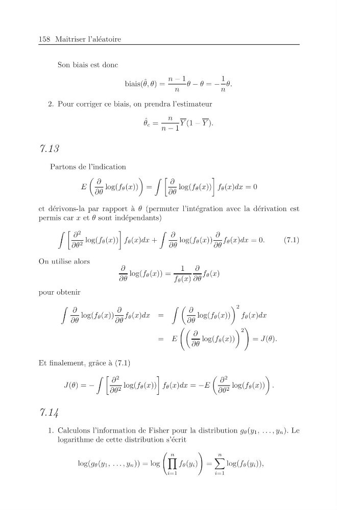
158 Maˆ ıtriser l’al´ eatoire
Son biais est donc
biais( ˆ
θ, θ) =
n − 1
n
θ − θ = −
1
n
θ.
2. Pour corriger ce biais, on prendra l’estimateur
ˆ
θ c =
n
n − 1
Y (1 − Y ).
7.13
Partons de l’indication
E
∂
∂θ
log(f θ (x))
=
∂
∂θ
log(f θ (x))
f θ (x)dx = 0
et d´ erivons-la par rapport ` a θ (permuter l’int´ egration avec la d´ erivation est
permis car x et θ sont ind´ ependants)
∂
2
∂θ 2 log(f θ (x))
f θ (x)dx +
∂
∂θ
log(f θ (x))
∂
∂θ
f θ (x)dx = 0.
(7.1)
On utilise alors
∂
∂θ
log(f θ (x)) =
1
f θ (x)
∂
∂θ
f θ (x)
pour obtenir
∂
∂θ
log(f θ (x))
∂
∂θ
f θ (x)dx =
∂
∂θ
log(f θ (x))
2
f θ (x)dx
= E
∂
∂θ
log(f θ (x))
2
= J(θ).
Et finalement, grˆ ace ` a (7.1)
J(θ) = −
∂
2
∂θ 2 log(f θ (x))
f θ (x)dx = −E
∂
2
∂θ 2 log(f θ (x))
.
7.14
1. Calculons l’information de Fisher pour la distribution g θ (y 1 , . . . , y n ). Le
logarithme de cette distribution s’´ ecrit
log(g θ (y 1 , . . . , y n )) = log
n
i=1
f θ (y i )
=
n
i=1
log(f θ (y i )),