

1 It is easy to use arbitrary values on a computer; we could also use 1 km or 1
furlong. Finding a physical 1 km string is another matter . . .
Displacement
4
2
0
−2
−4
Direct
arrival T = 0.5
Synthetic seismogram for string
1
2
3
0
1.2
0.2
0.4
0.6
0.8
1
Time
Source
Receiver
Left
reflection T = 0.9
Right
reflection T = 1.1
x = 1
x = 0
x = 0.2
x = 0.7
1
2
3
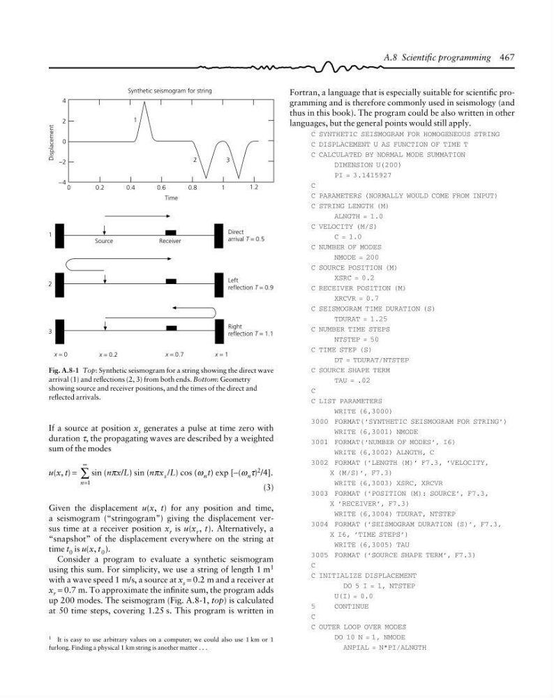
Fig. A.8-1 Top: Synthetic seismogram for a string showing the direct wave
arrival (1) and reflections (2, 3) from both ends. Bottom: Geometry
showing source and receiver positions, and the times of the direct and
reflected arrivals.
Fortran, a language that is especially suitable for scientific programming and is therefore commonly used in seismology (and
thus in this book). The program could be also written in other
languages, but the general points would still apply.
C SYNTHETIC SEISMOGRAM FOR HOMOGENEOUS STRING
C DISPLACEMENT U AS FUNCTION OF TIME T
C CALCULATED BY NORMAL MODE SUMMATION
DIMENSION U(200)
PI = 3.1415927
C
C PARAMETERS (NORMALLY WOULD COME FROM INPUT)
C STRING LENGTH (M)
ALNGTH = 1.0
C VELOCITY (M/S)
C = 1.0
C NUMBER OF MODES
NMODE = 200
C SOURCE POSITION (M)
XSRC = 0.2
C RECEIVER POSITION (M)
XRCVR = 0.7
C SEISMOGRAM TIME DURATION (S)
TDURAT = 1.25
C NUMBER TIME STEPS
NTSTEP = 50
C TIME STEP (S)
DT = TDURAT/NTSTEP
C SOURCE SHAPE TERM
TAU = .02
C
C LIST PARAMETERS
WRITE (6,3000)
3000 FORMAT(‘SYNTHETIC SEISMOGRAM FOR STRING’)
WRITE (6,3001) NMODE
3001 FORMAT(‘NUMBER OF MODES’, I6)
WRITE (6,3002) ALNGTH, C
3002 FORMAT (’LENGTH (M)’ F7.3, ‘VELOCITY,
X (M/S)’, F7.3)
WRITE (6,3003) XSRC, XRCVR
3003 FORMAT (’POSITION (M): SOURCE’, F7.3,
X ’RECEIVER’, F7.3)
WRITE (6,3004) TDURAT, NTSTEP
3004 FORMAT (’SEISMOGRAM DURATION (S)’, F7.3,
X I6, ’TIME STEPS’)
WRITE (6,3005) TAU
3005 FORMAT (’SOURCE SHAPE TERM’, F7.3)
C
C INITIALIZE DISPLACEMENT
DO 5 I = 1, NTSTEP
U(I) = 0.0
5
CONTINUE
C
C OUTER LOOP OVER MODES
DO 10 N = 1, NMODE
ANPIAL = N*PI/ALNGTH
If a source at position x s generates a pulse at time zero with
duration τ, the propagating waves are described by a weighted
sum of the modes
u(x, t) =
n=
∞
∑
1
sin (nπx/L) sin (nπx s /L) cos (ω n t) exp [−(ω n τ) 2 /4].
(3)
Given the displacement u(x, t) for any position and time,
a seismogram (“stringogram”) giving the displacement versus time at a receiver position x r is u(x r , t). Alternatively, a
“snapshot” of the displacement everywhere on the string at
time t 0 is u(x, t 0 ).
Consider a program to evaluate a synthetic seismogram
using this sum. For simplicity, we use a string of length 1 m
1
with a wave speed 1 m/s, a source at x s = 0.2 m and a receiver at
x r = 0.7 m. To approximate the infinite sum, the program adds
up 200 modes. The seismogram (Fig. A.8-1, top) is calculated
at 50 time steps, covering 1.25 s. This program is written in
A.8 Scientific programming 467
furlong. Finding a physical 1 km string is another matter . . .
Displacement
4
2
0
−2
−4
Direct
arrival T = 0.5
Synthetic seismogram for string
1
2
3
0
1.2
0.2
0.4
0.6
0.8
1
Time
Source
Receiver
Left
reflection T = 0.9
Right
reflection T = 1.1
x = 1
x = 0
x = 0.2
x = 0.7
1
2
3
Fig. A.8-1 Top: Synthetic seismogram for a string showing the direct wave
arrival (1) and reflections (2, 3) from both ends. Bottom: Geometry
showing source and receiver positions, and the times of the direct and
reflected arrivals.
Fortran, a language that is especially suitable for scientific programming and is therefore commonly used in seismology (and
thus in this book). The program could be also written in other
languages, but the general points would still apply.
C SYNTHETIC SEISMOGRAM FOR HOMOGENEOUS STRING
C DISPLACEMENT U AS FUNCTION OF TIME T
C CALCULATED BY NORMAL MODE SUMMATION
DIMENSION U(200)
PI = 3.1415927
C
C PARAMETERS (NORMALLY WOULD COME FROM INPUT)
C STRING LENGTH (M)
ALNGTH = 1.0
C VELOCITY (M/S)
C = 1.0
C NUMBER OF MODES
NMODE = 200
C SOURCE POSITION (M)
XSRC = 0.2
C RECEIVER POSITION (M)
XRCVR = 0.7
C SEISMOGRAM TIME DURATION (S)
TDURAT = 1.25
C NUMBER TIME STEPS
NTSTEP = 50
C TIME STEP (S)
DT = TDURAT/NTSTEP
C SOURCE SHAPE TERM
TAU = .02
C
C LIST PARAMETERS
WRITE (6,3000)
3000 FORMAT(‘SYNTHETIC SEISMOGRAM FOR STRING’)
WRITE (6,3001) NMODE
3001 FORMAT(‘NUMBER OF MODES’, I6)
WRITE (6,3002) ALNGTH, C
3002 FORMAT (’LENGTH (M)’ F7.3, ‘VELOCITY,
X (M/S)’, F7.3)
WRITE (6,3003) XSRC, XRCVR
3003 FORMAT (’POSITION (M): SOURCE’, F7.3,
X ’RECEIVER’, F7.3)
WRITE (6,3004) TDURAT, NTSTEP
3004 FORMAT (’SEISMOGRAM DURATION (S)’, F7.3,
X I6, ’TIME STEPS’)
WRITE (6,3005) TAU
3005 FORMAT (’SOURCE SHAPE TERM’, F7.3)
C
C INITIALIZE DISPLACEMENT
DO 5 I = 1, NTSTEP
U(I) = 0.0
5
CONTINUE
C
C OUTER LOOP OVER MODES
DO 10 N = 1, NMODE
ANPIAL = N*PI/ALNGTH
If a source at position x s generates a pulse at time zero with
duration τ, the propagating waves are described by a weighted
sum of the modes
u(x, t) =
n=
∞
∑
1
sin (nπx/L) sin (nπx s /L) cos (ω n t) exp [−(ω n τ) 2 /4].
(3)
Given the displacement u(x, t) for any position and time,
a seismogram (“stringogram”) giving the displacement versus time at a receiver position x r is u(x r , t). Alternatively, a
“snapshot” of the displacement everywhere on the string at
time t 0 is u(x, t 0 ).
Consider a program to evaluate a synthetic seismogram
using this sum. For simplicity, we use a string of length 1 m
1
with a wave speed 1 m/s, a source at x s = 0.2 m and a receiver at
x r = 0.7 m. To approximate the infinite sum, the program adds
up 200 modes. The seismogram (Fig. A.8-1, top) is calculated
at 50 time steps, covering 1.25 s. This program is written in
A.8 Scientific programming 467