

466 Appendix
r
r sin d
θ φ
dθ
θ
φ
dφ
dr
r sinθ
Spherical coordinates:
dV = r 2 sin dr d dφ
θ
θ
dS = r 2 sin d d
θ
φ
θ
dφ
r dθ
A.8 Scientific programming
Most seismological applications require computers, and these
requirements, especially in exploration applications with very
large data volumes, have spurred the development of computer
software and hardware. Some remarks about the use of computers in seismology thus seem appropriate.
Computer usage in seismology includes several broad and
overlapping categories:
• Computers are often used in data acquisition and recording systems.
• Data are initially displayed and manipulated using
computers.
• Subsequent analysis is frequently done using computers.
For example, seismograms can be filtered to enhance
certain frequencies or combined to better resolve certain
features.
• Theoretical, or synthetic, seismograms are often computed for a range of the parameters under study and compared to data to find the best fit.
• Computers are used to invert seismological data to determine the parameters of a model which best matches the
data.
• Computer modeling is often used to draw geological inferences from seismological observations. For example,
seismic velocity data are compared to the predictions of
models for the velocity of rock as a function of composition, temperature, and pressure.
These applications often require scientific programming, a
programming style used for essentially mathematical applications. Some problems in this book also require scientific programming. Although programming is a matter of personal
style, this section discusses several points that may be helpful.
The suggested reading provides some starting points for readers interested in pursuing these topics further.
A.8.1 Example: synthetic seismogram calculation
Consider a program to compute a synthetic seismogram for
waves in a one-dimensional constant-velocity medium, a mathematically idealized string that illustrates features of wave
behavior. The program is based on u(x, t), the displacement as
a function of position x and time t. The displacement is zero at
the fixed ends of the string, x = 0 and x = L, between which
waves travel at speed v. As in Section 2.2.5, the displacement
can be written as the sum of the normal modes of the string,
each of which is a standing wave with n half wavelengths along
the string,
u n (x, t) = sin (nπx/L) cos (ω n t),
(1)
and vibrates at a characteristic frequency, or eigenfrequency,
ω n = nπv/L.
(2)
curl
sin
(sin
)
u ê
=
−
⎛
⎝
⎜
⎞
⎠
⎟
r r
u
u
1
θ
θ
θ
φ
φ
θ
∂
∂
∂
∂
+
−
⎛
⎝
⎜
⎞
⎠
⎟
sin
sin
( )
ê θ
φ
θ
φ
θ
1
r
u
r
ru
r
∂
∂
∂
∂
+
−
⎛
⎝
⎜
⎞
⎠
⎟
( )
ê φ
θ
θ
1
r
r
ru
u r
∂
∂
∂
∂
(16)
∇ =
⎛
⎝
⎜
⎞
⎠
⎟ +
⎛
⎝
⎜
⎞
⎠
⎟
2
2
2
2
1
1
ψ
ψ
θ θ
θ
ψ
θ
sin
sin
r
r
r
r
r
∂
∂
∂
∂
∂
∂
∂
∂
+
sin
.
1
2
2
2
2
r
θ
ψ
φ
∂
∂
(17)
These expressions are used when we discuss spherical waves in
Section 2.4 and the earth’s normal modes in Section 2.9.
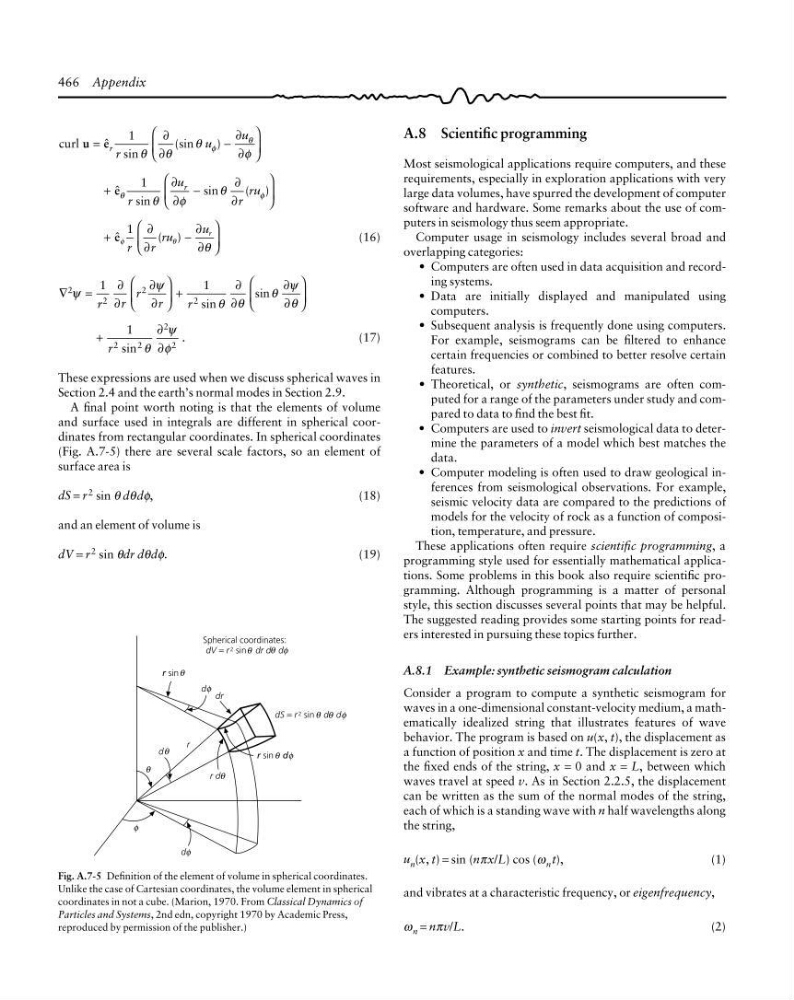
A final point worth noting is that the elements of volume
and surface used in integrals are different in spherical coordinates from rectangular coordinates. In spherical coordinates
(Fig. A.7-5) there are several scale factors, so an element of
surface area is
dS = r 2 sin θ dθdφ,
(18)
and an element of volume is
dV = r 2 sin θdr dθdφ.
(19)
Fig. A.7-5 Definition of the element of volume in spherical coordinates.
Unlike the case of Cartesian coordinates, the volume element in spherical
coordinates in not a cube. (Marion, 1970. From Classical Dynamics of
Particles and Systems, 2nd edn, copyright 1970 by Academic Press,
reproduced by permission of the publisher.)
r
r sin d
θ φ
dθ
θ
φ
dφ
dr
r sinθ
Spherical coordinates:
dV = r 2 sin dr d dφ
θ
θ
dS = r 2 sin d d
θ
φ
θ
dφ
r dθ
A.8 Scientific programming
Most seismological applications require computers, and these
requirements, especially in exploration applications with very
large data volumes, have spurred the development of computer
software and hardware. Some remarks about the use of computers in seismology thus seem appropriate.
Computer usage in seismology includes several broad and
overlapping categories:
• Computers are often used in data acquisition and recording systems.
• Data are initially displayed and manipulated using
computers.
• Subsequent analysis is frequently done using computers.
For example, seismograms can be filtered to enhance
certain frequencies or combined to better resolve certain
features.
• Theoretical, or synthetic, seismograms are often computed for a range of the parameters under study and compared to data to find the best fit.
• Computers are used to invert seismological data to determine the parameters of a model which best matches the
data.
• Computer modeling is often used to draw geological inferences from seismological observations. For example,
seismic velocity data are compared to the predictions of
models for the velocity of rock as a function of composition, temperature, and pressure.
These applications often require scientific programming, a
programming style used for essentially mathematical applications. Some problems in this book also require scientific programming. Although programming is a matter of personal
style, this section discusses several points that may be helpful.
The suggested reading provides some starting points for readers interested in pursuing these topics further.
A.8.1 Example: synthetic seismogram calculation
Consider a program to compute a synthetic seismogram for
waves in a one-dimensional constant-velocity medium, a mathematically idealized string that illustrates features of wave
behavior. The program is based on u(x, t), the displacement as
a function of position x and time t. The displacement is zero at
the fixed ends of the string, x = 0 and x = L, between which
waves travel at speed v. As in Section 2.2.5, the displacement
can be written as the sum of the normal modes of the string,
each of which is a standing wave with n half wavelengths along
the string,
u n (x, t) = sin (nπx/L) cos (ω n t),
(1)
and vibrates at a characteristic frequency, or eigenfrequency,
ω n = nπv/L.
(2)
curl
sin
(sin
)
u ê
=
−
⎛
⎝
⎜
⎞
⎠
⎟
r r
u
u
1
θ
θ
θ
φ
φ
θ
∂
∂
∂
∂
+
−
⎛
⎝
⎜
⎞
⎠
⎟
sin
sin
( )
ê θ
φ
θ
φ
θ
1
r
u
r
ru
r
∂
∂
∂
∂
+
−
⎛
⎝
⎜
⎞
⎠
⎟
( )
ê φ
θ
θ
1
r
r
ru
u r
∂
∂
∂
∂
(16)
∇ =
⎛
⎝
⎜
⎞
⎠
⎟ +
⎛
⎝
⎜
⎞
⎠
⎟
2
2
2
2
1
1
ψ
ψ
θ θ
θ
ψ
θ
sin
sin
r
r
r
r
r
∂
∂
∂
∂
∂
∂
∂
∂
+
sin
.
1
2
2
2
2
r
θ
ψ
φ
∂
∂
(17)
These expressions are used when we discuss spherical waves in
Section 2.4 and the earth’s normal modes in Section 2.9.
A final point worth noting is that the elements of volume
and surface used in integrals are different in spherical coordinates from rectangular coordinates. In spherical coordinates
(Fig. A.7-5) there are several scale factors, so an element of
surface area is
dS = r 2 sin θ dθdφ,
(18)
and an element of volume is
dV = r 2 sin θdr dθdφ.
(19)
Fig. A.7-5 Definition of the element of volume in spherical coordinates.
Unlike the case of Cartesian coordinates, the volume element in spherical
coordinates in not a cube. (Marion, 1970. From Classical Dynamics of
Particles and Systems, 2nd edn, copyright 1970 by Academic Press,
reproduced by permission of the publisher.)