

468 Appendix
C SPACE TERMS: SOURCE AND RECEIVER
SXS = SIN(ANPIAL*XSRC)
SXR = SIN(ANPIAL*XRCVR)
C MODE FREQUENCY
WN = N*PI*C/ALNGTH
C TIME INDEPENDENT TERMS
DMP = (TAU*WN)**2
SCALE = EXP(-DMP/4.)
SPACE = SXS*SXR*SCALE
C
C INNER LOOP OVER TIME STEPS
DO 15 J = 1, NTSTEP
T = DT*(J – 1)
CWT = COS(WN*T)
C COMPUTE DISPLACEMENT
U(J) = U(J) + CWT*SPACE
15
CONTINUE
10
CONTINUE
C
C OUTPUT SEISMOGRAM FOR LATER PLOTTING
WRITE (6, 3101)(U(J), J = 1, NTSTEP)
3101 FORMAT (7F10.4)
STOP
END
This example brings out several points:
• Is the answer correct? Two different types of error occur
in scientific programs. First, the program may be wrong. In
this case, the mathematical formulation correctly describes the
physical problem, but the program incorrectly implements
this formulation. This is the usual situation, in which “bugs”
are identified and corrected. Second, the formulation may be
wrong, so the program correctly implements an incorrect
mathematical model. This could occur because of a mathematical error, like an attempt to sum a divergent series, or a physical
error, such as an equation that does not correctly describe
waves on a string. An incorrect formulation is particularly disturbing because it cannot be detected by checking the program.
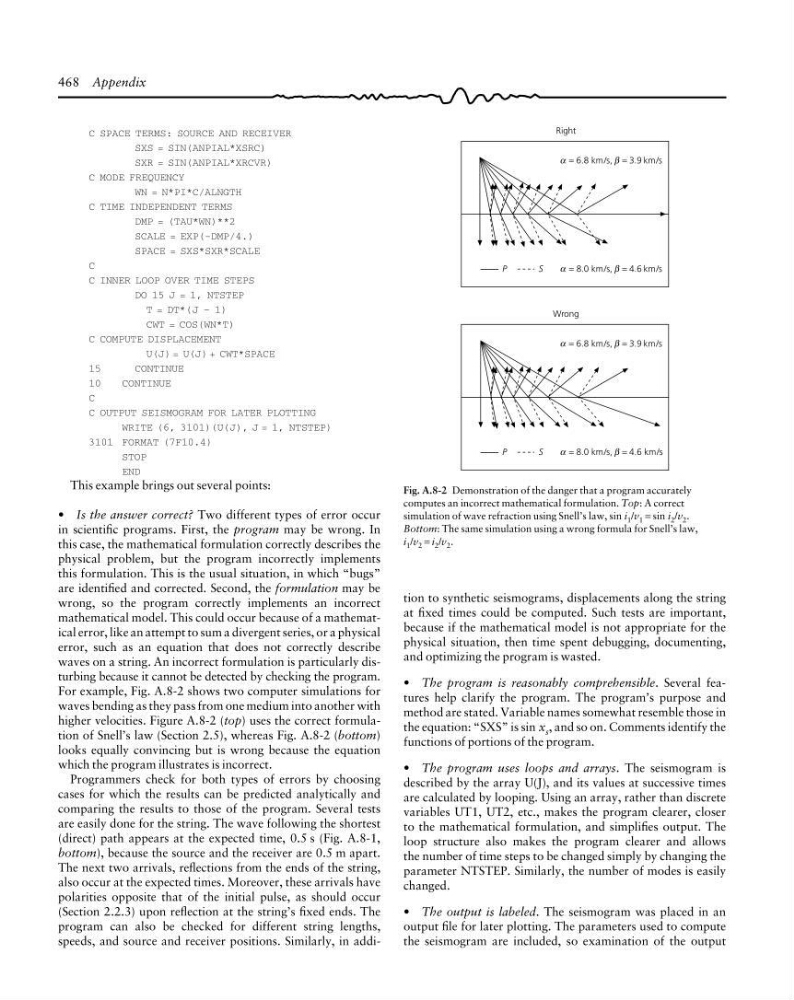
For example, Fig. A.8-2 shows two computer simulations for
waves bending as they pass from one medium into another with
higher velocities. Figure A.8-2 (top) uses the correct formulation of Snell’s law (Section 2.5), whereas Fig. A.8-2 (bottom)
looks equally convincing but is wrong because the equation
which the program illustrates is incorrect.
Programmers check for both types of errors by choosing
cases for which the results can be predicted analytically and
comparing the results to those of the program. Several tests
are easily done for the string. The wave following the shortest
(direct) path appears at the expected time, 0.5 s (Fig. A.8-1,
bottom), because the source and the receiver are 0.5 m apart.
The next two arrivals, reflections from the ends of the string,
also occur at the expected times. Moreover, these arrivals have
polarities opposite that of the initial pulse, as should occur
(Section 2.2.3) upon reflection at the string’s fixed ends. The
program can also be checked for different string lengths,
speeds, and source and receiver positions. Similarly, in addiFig. A.8-2 Demonstration of the danger that a program accurately
computes an incorrect mathematical formulation. Top: A correct
simulation of wave refraction using Snell’s law, sin i 1 /v 1 = sin i 2 /v 2 .
Bottom: The same simulation using a wrong formula for Snell’s law,
i 1 /v 2 = i 2 /v 2 .
P
Right
S
Wrong
= 6.8 km/s, = 3.9 km/s
α
β
= 8.0 km/s, = 4.6 km/s
α
β
P
S
= 6.8 km/s, = 3.9 km/s
α
β
= 8.0 km/s, = 4.6 km/s
α
β
tion to synthetic seismograms, displacements along the string
at fixed times could be computed. Such tests are important,
because if the mathematical model is not appropriate for the
physical situation, then time spent debugging, documenting,
and optimizing the program is wasted.
• The program is reasonably comprehensible. Several features help clarify the program. The program’s purpose and
method are stated. Variable names somewhat resemble those in
the equation: “SXS” is sin x s , and so on. Comments identify the
functions of portions of the program.
• The program uses loops and arrays. The seismogram is
described by the array U(J), and its values at successive times
are calculated by looping. Using an array, rather than discrete
variables UT1, UT2, etc., makes the program clearer, closer
to the mathematical formulation, and simplifies output. The
loop structure also makes the program clearer and allows
the number of time steps to be changed simply by changing the
parameter NTSTEP. Similarly, the number of modes is easily
changed.
• The output is labeled. The seismogram was placed in an
output file for later plotting. The parameters used to compute
the seismogram are included, so examination of the output
C SPACE TERMS: SOURCE AND RECEIVER
SXS = SIN(ANPIAL*XSRC)
SXR = SIN(ANPIAL*XRCVR)
C MODE FREQUENCY
WN = N*PI*C/ALNGTH
C TIME INDEPENDENT TERMS
DMP = (TAU*WN)**2
SCALE = EXP(-DMP/4.)
SPACE = SXS*SXR*SCALE
C
C INNER LOOP OVER TIME STEPS
DO 15 J = 1, NTSTEP
T = DT*(J – 1)
CWT = COS(WN*T)
C COMPUTE DISPLACEMENT
U(J) = U(J) + CWT*SPACE
15
CONTINUE
10
CONTINUE
C
C OUTPUT SEISMOGRAM FOR LATER PLOTTING
WRITE (6, 3101)(U(J), J = 1, NTSTEP)
3101 FORMAT (7F10.4)
STOP
END
This example brings out several points:
• Is the answer correct? Two different types of error occur
in scientific programs. First, the program may be wrong. In
this case, the mathematical formulation correctly describes the
physical problem, but the program incorrectly implements
this formulation. This is the usual situation, in which “bugs”
are identified and corrected. Second, the formulation may be
wrong, so the program correctly implements an incorrect
mathematical model. This could occur because of a mathematical error, like an attempt to sum a divergent series, or a physical
error, such as an equation that does not correctly describe
waves on a string. An incorrect formulation is particularly disturbing because it cannot be detected by checking the program.
For example, Fig. A.8-2 shows two computer simulations for
waves bending as they pass from one medium into another with
higher velocities. Figure A.8-2 (top) uses the correct formulation of Snell’s law (Section 2.5), whereas Fig. A.8-2 (bottom)
looks equally convincing but is wrong because the equation
which the program illustrates is incorrect.
Programmers check for both types of errors by choosing
cases for which the results can be predicted analytically and
comparing the results to those of the program. Several tests
are easily done for the string. The wave following the shortest
(direct) path appears at the expected time, 0.5 s (Fig. A.8-1,
bottom), because the source and the receiver are 0.5 m apart.
The next two arrivals, reflections from the ends of the string,
also occur at the expected times. Moreover, these arrivals have
polarities opposite that of the initial pulse, as should occur
(Section 2.2.3) upon reflection at the string’s fixed ends. The
program can also be checked for different string lengths,
speeds, and source and receiver positions. Similarly, in addiFig. A.8-2 Demonstration of the danger that a program accurately
computes an incorrect mathematical formulation. Top: A correct
simulation of wave refraction using Snell’s law, sin i 1 /v 1 = sin i 2 /v 2 .
Bottom: The same simulation using a wrong formula for Snell’s law,
i 1 /v 2 = i 2 /v 2 .
P
Right
S
Wrong
= 6.8 km/s, = 3.9 km/s
α
β
= 8.0 km/s, = 4.6 km/s
α
β
P
S
= 6.8 km/s, = 3.9 km/s
α
β
= 8.0 km/s, = 4.6 km/s
α
β
tion to synthetic seismograms, displacements along the string
at fixed times could be computed. Such tests are important,
because if the mathematical model is not appropriate for the
physical situation, then time spent debugging, documenting,
and optimizing the program is wasted.
• The program is reasonably comprehensible. Several features help clarify the program. The program’s purpose and
method are stated. Variable names somewhat resemble those in
the equation: “SXS” is sin x s , and so on. Comments identify the
functions of portions of the program.
• The program uses loops and arrays. The seismogram is
described by the array U(J), and its values at successive times
are calculated by looping. Using an array, rather than discrete
variables UT1, UT2, etc., makes the program clearer, closer
to the mathematical formulation, and simplifies output. The
loop structure also makes the program clearer and allows
the number of time steps to be changed simply by changing the
parameter NTSTEP. Similarly, the number of modes is easily
changed.
• The output is labeled. The seismogram was placed in an
output file for later plotting. The parameters used to compute
the seismogram are included, so examination of the output