

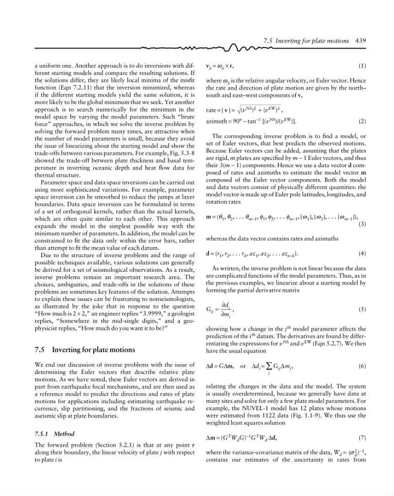
a uniform one. Another approach is to do inversions with different starting models and compare the resulting solutions. If
the solutions differ, they are likely local minima of the misfit
function (Eqn 7.2.11) that the inversion minimized, whereas
if the different starting models yield the same solution, it is
more likely to be the global minimum that we seek. Yet another
approach is to search numerically for the minimum in the
model space by varying the model parameters. Such “brute
force” approaches, in which we solve the inverse problem by
solving the forward problem many times, are attractive when
the number of model parameters is small, because they avoid
the issue of linearizing about the starting model and show the
trade-offs between various parameters. For example, Fig. 5.3-8
showed the trade-off between plate thickness and basal temperature in inverting oceanic depth and heat flow data for
thermal structure.
Parameter space and data space inversions can be carried out
using more sophisticated variations. For example, parameter
space inversion can be smoothed to reduce the jumps at layer
boundaries. Data space inversion can be formulated in terms
of a set of orthogonal kernels, rather than the actual kernels,
which are often quite similar to each other. This approach
expands the model in the simplest possible way with the
minimum number of parameters. In addition, the model can be
constrained to fit the data only within the error bars, rather
than attempt to fit the mean value of each datum.
Due to the structure of inverse problems and the range of
possible techniques available, various solutions can generally
be derived for a set of seismological observations. As a result,
inverse problems remain an important research area. The
choices, ambiguities, and trade-offs in the solutions of these
problems are sometimes key features of the solution. Attempts
to explain these issues can be frustrating to nonseismologists,
as illustrated by the joke that in response to the question
“How much is 2 + 2,” an engineer replies “3.9999,” a geologist
replies, “Somewhere in the mid-single digits,” and a geophysicist replies, “How much do you want it to be?”
7.5 Inverting for plate motions
We end our discussion of inverse problems with the issue of
determining the Euler vectors that describe relative plate
motions. As we have noted, these Euler vectors are derived in
part from earthquake focal mechanisms, and are then used as
a reference model to predict the directions and rates of plate
motions for applications including estimating earthquake recurrence, slip partitioning, and the fractions of seismic and
aseismic slip at plate boundaries.
7.5.1 Method
The forward problem (Section 5.2.1) is that at any point r
along their boundary, the linear velocity of plate j with respect
to plate i is
v ji = ω ji × r,
(1)
where ω ji is the relative angular velocity, or Euler vector. Hence
the rate and direction of plate motion are given by the north–
south and east–west components of v,
rate = | v | = (
)
(
) ,
v
v
NS
EW
2
2
+
azimuth = 90° − tan
−1 [(v
NS )/(v
EW )].
(2)
The corresponding inverse problem is to find a model, or
set of Euler vectors, that best predicts the observed motions.
Because Euler vectors can be added, assuming that the plates
are rigid, m plates are specified by m − 1 Euler vectors, and thus
their 3(m − 1) components. Hence we use a data vector d composed of rates and azimuths to estimate the model vector m
composed of the Euler vector components. Both the model
and data vectors consist of physically different quantities: the
model vector is made up of Euler pole latitudes, longitudes, and
rotation rates
m = (θ 1 , θ 2 , . . . θ m−1 , φ 1 , φ 2 , . . . φ m−1 , | ω 1 |, | ω 2 |, . . . | ω m−1 |),
(3)
whereas the data vector contains rates and azimuths
d = (r 1 , r 2 , . . . r k , az 1 , az 2 , . . . az n−k ).
(4)
As written, the inverse problem is not linear because the data
are complicated functions of the model parameters. Thus, as in
the previous examples, we linearize about a starting model by
forming the partial derivative matrix
G
d
m
ij
i
j
=
,
∂
∂
(5)
showing how a change in the j th model parameter affects the
prediction of the i
th datum. The derivatives are found by differentiating the expressions for v NS and v EW (Eqn 5.2.7). We then
have the usual equation
∆d = G∆m, or ∆d i =
j
∑ G ij ∆m j ,
(6)
relating the changes in the data and the model. The system
is usually overdetermined, because we generally have data at
many sites and solve for only a few plate model parameters. For
example, the NUVEL-1 model has 12 plates whose motions
were estimated from 1122 data (Fig. 1.1-9). We thus use the
weighted least squares solution
∆m = (G T W d G) −1 G T W d ∆d,
(7)
where the variance–covariance matrix of the data, W d = ( )
σ d
2 1
− ,
contains our estimates of the uncertainty in rates from
7.5 Inverting for plate motions 439
the solutions differ, they are likely local minima of the misfit
function (Eqn 7.2.11) that the inversion minimized, whereas
if the different starting models yield the same solution, it is
more likely to be the global minimum that we seek. Yet another
approach is to search numerically for the minimum in the
model space by varying the model parameters. Such “brute
force” approaches, in which we solve the inverse problem by
solving the forward problem many times, are attractive when
the number of model parameters is small, because they avoid
the issue of linearizing about the starting model and show the
trade-offs between various parameters. For example, Fig. 5.3-8
showed the trade-off between plate thickness and basal temperature in inverting oceanic depth and heat flow data for
thermal structure.
Parameter space and data space inversions can be carried out
using more sophisticated variations. For example, parameter
space inversion can be smoothed to reduce the jumps at layer
boundaries. Data space inversion can be formulated in terms
of a set of orthogonal kernels, rather than the actual kernels,
which are often quite similar to each other. This approach
expands the model in the simplest possible way with the
minimum number of parameters. In addition, the model can be
constrained to fit the data only within the error bars, rather
than attempt to fit the mean value of each datum.
Due to the structure of inverse problems and the range of
possible techniques available, various solutions can generally
be derived for a set of seismological observations. As a result,
inverse problems remain an important research area. The
choices, ambiguities, and trade-offs in the solutions of these
problems are sometimes key features of the solution. Attempts
to explain these issues can be frustrating to nonseismologists,
as illustrated by the joke that in response to the question
“How much is 2 + 2,” an engineer replies “3.9999,” a geologist
replies, “Somewhere in the mid-single digits,” and a geophysicist replies, “How much do you want it to be?”
7.5 Inverting for plate motions
We end our discussion of inverse problems with the issue of
determining the Euler vectors that describe relative plate
motions. As we have noted, these Euler vectors are derived in
part from earthquake focal mechanisms, and are then used as
a reference model to predict the directions and rates of plate
motions for applications including estimating earthquake recurrence, slip partitioning, and the fractions of seismic and
aseismic slip at plate boundaries.
7.5.1 Method
The forward problem (Section 5.2.1) is that at any point r
along their boundary, the linear velocity of plate j with respect
to plate i is
v ji = ω ji × r,
(1)
where ω ji is the relative angular velocity, or Euler vector. Hence
the rate and direction of plate motion are given by the north–
south and east–west components of v,
rate = | v | = (
)
(
) ,
v
v
NS
EW
2
2
+
azimuth = 90° − tan
−1 [(v
NS )/(v
EW )].
(2)
The corresponding inverse problem is to find a model, or
set of Euler vectors, that best predicts the observed motions.
Because Euler vectors can be added, assuming that the plates
are rigid, m plates are specified by m − 1 Euler vectors, and thus
their 3(m − 1) components. Hence we use a data vector d composed of rates and azimuths to estimate the model vector m
composed of the Euler vector components. Both the model
and data vectors consist of physically different quantities: the
model vector is made up of Euler pole latitudes, longitudes, and
rotation rates
m = (θ 1 , θ 2 , . . . θ m−1 , φ 1 , φ 2 , . . . φ m−1 , | ω 1 |, | ω 2 |, . . . | ω m−1 |),
(3)
whereas the data vector contains rates and azimuths
d = (r 1 , r 2 , . . . r k , az 1 , az 2 , . . . az n−k ).
(4)
As written, the inverse problem is not linear because the data
are complicated functions of the model parameters. Thus, as in
the previous examples, we linearize about a starting model by
forming the partial derivative matrix
G
d
m
ij
i
j
=
,
∂
∂
(5)
showing how a change in the j th model parameter affects the
prediction of the i
th datum. The derivatives are found by differentiating the expressions for v NS and v EW (Eqn 5.2.7). We then
have the usual equation
∆d = G∆m, or ∆d i =
j
∑ G ij ∆m j ,
(6)
relating the changes in the data and the model. The system
is usually overdetermined, because we generally have data at
many sites and solve for only a few plate model parameters. For
example, the NUVEL-1 model has 12 plates whose motions
were estimated from 1122 data (Fig. 1.1-9). We thus use the
weighted least squares solution
∆m = (G T W d G) −1 G T W d ∆d,
(7)
where the variance–covariance matrix of the data, W d = ( )
σ d
2 1
− ,
contains our estimates of the uncertainty in rates from
7.5 Inverting for plate motions 439