

440 Inverse Problems
= 100
1
0.8
0.6
0.4
0.2
0
3
P(
2
, )
χ
ν ν
0
1
2
χ 2 test
χ
2
ν
= 10
ν
ν
magnetic anomalies and the uncertainties in directions
associated with estimating transform azimuths and determining earthquake slip vectors. The weighted solution is
needed because the uncertainties have different dimensions and
vary between data points.
Thus uncertainties in the estimated Euler vectors are given by
the model variance–covariance matrix
σ 2
m = (G T W d G) −1 .
(8)
Uncertainties associated with the Euler poles are often shown
by error ellipses analogous to those for earthquake locations,
whereas those for the rates are quoted separately. Alternatively, we can view the pole and rate uncertainties as forming
a three-dimensional ellipsoid. Hence two Euler vectors are
distinct if their error ellipsoids do not overlap. As we have seen,
conventional global plate motion studies using magnetic
anomalies, transforms, and earthquake slip vectors yield solutions similar to those obtained by using the same formulation
to invert the rates and azimuths of plate motions determined by
space-based geodesy (Section 5.2.3). This agreement is gratifying, given that the conventional solutions combine data from
magnetic anomalies averaged over millions of years, the azimuths of transform faults that formed over long times, and the
slip vectors of earthquakes, whereas the space-geodetic solutions based on data spanning only a few years have different
uncertainties.
7.5.2 Testing the results with χ 2 and F-ratio tests
Given a model derived by inversion, the natural question is,
how good is it? This issue is a specific case of the general one
of testing how well a model fits data, which is discussed in
statistics texts. For our purposes we focus on two issues and
note some results without proof.
One common way to test how well a model fits data uses the
misfit function χ 2 that we minimized to derive the least squares
solution (Eqn 7.2.11). We write it as
χ
σ
2
2
2
=
−
∑
(
) ,
d d
i
i
m
i
i
(9)
where d i
m are the data predicted by the model, d i are the data
observed, and σ i are their uncertainties. Lower values of χ 2 correspond to better fits. However, because a model derived from
these data is bound to fit better than one derived without them,
we examine the reduced chi square
χ
2
ν = χ
2
/ν
(10)
where the parameter ν, known as the number of degrees of
freedom, equals n − p where n is the number of data and p is the
number of model parameters estimated in the inversion.
If the model is a good fit to the data and our estimates of the
uncertainties are reasonable, then we expect χ 2
ν to be around 1.
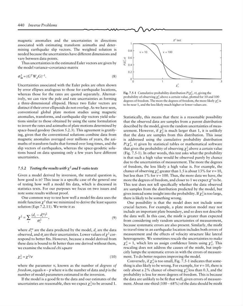
Fig. 7.5-1 Cumulative probability distribution P(χ 2
ν , ν), giving the
probability of observing χ
2
ν above a certain value, plotted for 10 and 100
degrees of freedom. The more the degrees of freedom, the more likely χ
2
ν is
to be near 1, and the less likely much higher or lower values are.
Statistically, this means that there is a reasonable possibility
that the observed data are samples from a parent distribution
described by the model, given the random uncertainties of measurement. However, if χ
2
ν is much larger than 1, it is unlikely
that the data are samples from this distribution. This issue
is addressed using the cumulative probability distribution
P(χ 2
ν , ν) given by statistical tables or mathematical software
that gives the probability of observing χ 2
ν above a certain value
(Fig. 7.5-1). In other words, this test asks what the probability
is that such a high value would be observed purely by chance
due to the uncertainties of measurement. The more the degrees
of freedom, the less likely a high value is. For example, the
chance of observing χ 2
ν greater than 1.5 is about 13% for ν = 10,
but less than 1% for ν = 100. Thus, the more data we have, the
more the degrees of freedom, and closer to 1 we expect χ 2 to be.
This test does not tell specifically whether the data observed
are samples from the distribution predicted by the model, but
gives instead some insight into the probability. If χ 2
ν is too large,
there is likely to be something wrong.
One possibility is that the model does not include some
crucial factors. For example, a plate motion model may not
include an important plate boundary, and so does not describe
the data well. In this case, the misfit is greater than expected
from considering only random uncertainties of measurement,
because systematic errors are also present. Similarly, the misfit
to travel time in an earthquake location includes both errors of
measurement and the effects of velocity structure like lateral
heterogeneity. We sometimes rescale the uncertainties to make
χ 2
ν = 1, which lets us assign confidence limits using χ 2
ν . This
rescaling does not address the causes of the misfit, but implicitly lumps the systematic errors in with the errors of measurement. To do better requires improving the model.
Conversely, if χ
2
ν is too small, Fig. 7.5-1 indicates that something is also likely to be wrong. For example, for ν = 10, there is
only about a 2% chance of observing χ 2
ν less than 0.3, and the
probability is less for more degrees of freedom. This is because
the data are unlikely to be fit that well, given errors of measurement. About one-third (100 − 68%) of the data should be misfit
= 100
1
0.8
0.6
0.4
0.2
0
3
P(
2
, )
χ
ν ν
0
1
2
χ 2 test
χ
2
ν
= 10
ν
ν
magnetic anomalies and the uncertainties in directions
associated with estimating transform azimuths and determining earthquake slip vectors. The weighted solution is
needed because the uncertainties have different dimensions and
vary between data points.
Thus uncertainties in the estimated Euler vectors are given by
the model variance–covariance matrix
σ 2
m = (G T W d G) −1 .
(8)
Uncertainties associated with the Euler poles are often shown
by error ellipses analogous to those for earthquake locations,
whereas those for the rates are quoted separately. Alternatively, we can view the pole and rate uncertainties as forming
a three-dimensional ellipsoid. Hence two Euler vectors are
distinct if their error ellipsoids do not overlap. As we have seen,
conventional global plate motion studies using magnetic
anomalies, transforms, and earthquake slip vectors yield solutions similar to those obtained by using the same formulation
to invert the rates and azimuths of plate motions determined by
space-based geodesy (Section 5.2.3). This agreement is gratifying, given that the conventional solutions combine data from
magnetic anomalies averaged over millions of years, the azimuths of transform faults that formed over long times, and the
slip vectors of earthquakes, whereas the space-geodetic solutions based on data spanning only a few years have different
uncertainties.
7.5.2 Testing the results with χ 2 and F-ratio tests
Given a model derived by inversion, the natural question is,
how good is it? This issue is a specific case of the general one
of testing how well a model fits data, which is discussed in
statistics texts. For our purposes we focus on two issues and
note some results without proof.
One common way to test how well a model fits data uses the
misfit function χ 2 that we minimized to derive the least squares
solution (Eqn 7.2.11). We write it as
χ
σ
2
2
2
=
−
∑
(
) ,
d d
i
i
m
i
i
(9)
where d i
m are the data predicted by the model, d i are the data
observed, and σ i are their uncertainties. Lower values of χ 2 correspond to better fits. However, because a model derived from
these data is bound to fit better than one derived without them,
we examine the reduced chi square
χ
2
ν = χ
2
/ν
(10)
where the parameter ν, known as the number of degrees of
freedom, equals n − p where n is the number of data and p is the
number of model parameters estimated in the inversion.
If the model is a good fit to the data and our estimates of the
uncertainties are reasonable, then we expect χ 2
ν to be around 1.
Fig. 7.5-1 Cumulative probability distribution P(χ 2
ν , ν), giving the
probability of observing χ
2
ν above a certain value, plotted for 10 and 100
degrees of freedom. The more the degrees of freedom, the more likely χ
2
ν is
to be near 1, and the less likely much higher or lower values are.
Statistically, this means that there is a reasonable possibility
that the observed data are samples from a parent distribution
described by the model, given the random uncertainties of measurement. However, if χ
2
ν is much larger than 1, it is unlikely
that the data are samples from this distribution. This issue
is addressed using the cumulative probability distribution
P(χ 2
ν , ν) given by statistical tables or mathematical software
that gives the probability of observing χ 2
ν above a certain value
(Fig. 7.5-1). In other words, this test asks what the probability
is that such a high value would be observed purely by chance
due to the uncertainties of measurement. The more the degrees
of freedom, the less likely a high value is. For example, the
chance of observing χ 2
ν greater than 1.5 is about 13% for ν = 10,
but less than 1% for ν = 100. Thus, the more data we have, the
more the degrees of freedom, and closer to 1 we expect χ 2 to be.
This test does not tell specifically whether the data observed
are samples from the distribution predicted by the model, but
gives instead some insight into the probability. If χ 2
ν is too large,
there is likely to be something wrong.
One possibility is that the model does not include some
crucial factors. For example, a plate motion model may not
include an important plate boundary, and so does not describe
the data well. In this case, the misfit is greater than expected
from considering only random uncertainties of measurement,
because systematic errors are also present. Similarly, the misfit
to travel time in an earthquake location includes both errors of
measurement and the effects of velocity structure like lateral
heterogeneity. We sometimes rescale the uncertainties to make
χ 2
ν = 1, which lets us assign confidence limits using χ 2
ν . This
rescaling does not address the causes of the misfit, but implicitly lumps the systematic errors in with the errors of measurement. To do better requires improving the model.
Conversely, if χ
2
ν is too small, Fig. 7.5-1 indicates that something is also likely to be wrong. For example, for ν = 10, there is
only about a 2% chance of observing χ 2
ν less than 0.3, and the
probability is less for more degrees of freedom. This is because
the data are unlikely to be fit that well, given errors of measurement. About one-third (100 − 68%) of the data should be misfit