

438 Inverse Problems
0
50
100
150
200
250
300
350
400
Depth (km)
0
100
200
300
400
5.0
(a)
∂C/∂ and ∂U/∂ (× 10
−2 )
β
β
−10
−5
0
5
1 0
1 5
2 0
C 40
U 40
C 100
U 100
(b)
Shear velocity (km/s)
Depth (km)
4.8
3.8
4.0
4.2
4.4
4.6
starting model
inversion result
(c)
0
100
200
300
400
Depth (km)
−286
−173
−86
−
32−
−8
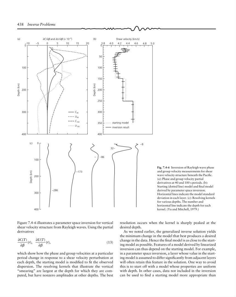
Figure 7.4-6 illustrates a parameter space inversion for vertical
shear velocity structure from Rayleigh waves. Using the partial
derivatives
∂
∂
∂
∂
C T r
U T r
( ) ( ),
( ) ( ),
β
β
(13)
which show how the phase and group velocities at a particular
period change in response to a shear velocity perturbation at
each depth, the starting model is modified to fit the observed
dispersion. The resolving kernels that illustrate the vertical
“smearing” are largest at the depth for which they are computed, but have nonzero amplitudes at other depths. The best
resolution occurs when the kernel is sharply peaked at the
desired depth.
As we noted earlier, the generalized inverse solution yields
the minimum change in the model that best produces a desired
change in the data. Hence the final model is as close to the starting model as possible. Features of a model derived by linearized
inversion can thus depend on the starting model. For example,
in a parameter space inversion, a layer whose value in the starting model is assumed to differ significantly from adjacent layers
will often retain this feature in the solution. One way to avoid
this is to start off with a model whose properties are uniform
with depth. In other cases, data not included in the inversion
can be used to find a starting model more appropriate than
Fig. 7.4-6 Inversion of Rayleigh wave phase
and group velocity measurements for shear
wave velocity structure beneath the Pacific.
(a): Phase and group velocity partial
derivatives at 40 and 100 s periods. (b):
Starting (dotted line) model and final model
derived by parameter space inversion.
Horizontal lines indicate the model standard
deviation in each layer. (c): Resolving kernels
for various depths. The number and
horizontal line indicate the depth for each
kernel. (Yu and Mitchell, 1979.)
0
50
100
150
200
250
300
350
400
Depth (km)
0
100
200
300
400
5.0
(a)
∂C/∂ and ∂U/∂ (× 10
−2 )
β
β
−10
−5
0
5
1 0
1 5
2 0
C 40
U 40
C 100
U 100
(b)
Shear velocity (km/s)
Depth (km)
4.8
3.8
4.0
4.2
4.4
4.6
starting model
inversion result
(c)
0
100
200
300
400
Depth (km)
−286
−173
−86
−
32−
−8
Figure 7.4-6 illustrates a parameter space inversion for vertical
shear velocity structure from Rayleigh waves. Using the partial
derivatives
∂
∂
∂
∂
C T r
U T r
( ) ( ),
( ) ( ),
β
β
(13)
which show how the phase and group velocities at a particular
period change in response to a shear velocity perturbation at
each depth, the starting model is modified to fit the observed
dispersion. The resolving kernels that illustrate the vertical
“smearing” are largest at the depth for which they are computed, but have nonzero amplitudes at other depths. The best
resolution occurs when the kernel is sharply peaked at the
desired depth.
As we noted earlier, the generalized inverse solution yields
the minimum change in the model that best produces a desired
change in the data. Hence the final model is as close to the starting model as possible. Features of a model derived by linearized
inversion can thus depend on the starting model. For example,
in a parameter space inversion, a layer whose value in the starting model is assumed to differ significantly from adjacent layers
will often retain this feature in the solution. One way to avoid
this is to start off with a model whose properties are uniform
with depth. In other cases, data not included in the inversion
can be used to find a starting model more appropriate than
Fig. 7.4-6 Inversion of Rayleigh wave phase
and group velocity measurements for shear
wave velocity structure beneath the Pacific.
(a): Phase and group velocity partial
derivatives at 40 and 100 s periods. (b):
Starting (dotted line) model and final model
derived by parameter space inversion.
Horizontal lines indicate the model standard
deviation in each layer. (c): Resolving kernels
for various depths. The number and
horizontal line indicate the depth for each
kernel. (Yu and Mitchell, 1979.)