

436 Inverse Problems
Data space
Layers
Parameter
space
Kernels
+
+
+ .
before, the generalized inverse gives the “best” solution in a
least squares sense. The concepts developed previously are useful for assessing the solution. Columns of the resolution
matrix, called resolving kernels, indicate how well the value in
the corresponding layer could be determined independently of
those in the other layers if the data had no errors. This uncertainty results from the inverse problem itself, and reflects the
best resolution possible, given the available kernels, analogous
to the resolution matrix (Eqn 7.3.23) in the tomographic example. It is also useful to consider the model covariance matrix,
which indicates the uncertainty in the model due to both the
nature of the inverse problem and the errors in the observations. Often a weighted average over a number of layers is the
best resolution obtainable, analogous to the blurring in travel
time tomography.
Parameter space inversion has a few unattractive features.
First, the layers in which attenuation is treated as constant must
be chosen in advance. This choice might not be a meaningful
one. Second, parametrizing the model as constant in these
layers yields a model with “steps” at layer boundaries. These
steps may be quite unphysical; in many cases our intuition
(admittedly sometimes a poor guide) suggests that physical
properties should vary smoothly with depth.
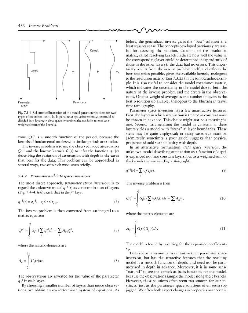
In an alternative formulation, data space inversion, the
unknown model describing attenuation as a function of depth
is expanded not into constant layers, but as a weighted sum of
the kernels themselves (Fig. 7.4-4, right),
q −1 (r) = ν j j
j
G r
( ).
∑
(9)
The inverse problem is then
Q
G r
G rdr
A
i
a
i
j j
j
ij j
j
− =
=
∑
∑
1
0
( )
( )
,
Ύ
ν
ν
(10)
where the matrix elements are
A ij
a
=
Ύ
0
G i (r)G j (r)dr.
(11)
The model is found by inverting for the expansion coefficients
ν j .
Data space inversion is less intuitive than parameter space
inversion, but has the attractive features that the resulting
model is a smooth function of depth, and need not be parametrized in depth in advance. Moreover, it is in some sense
“natural” to use the kernels as basis functions for the model,
because the observations sample the model along these kernels.
However, these solutions often seem too smooth for our instincts, just as the parameter space solutions often seem too
jagged. We often both expect changes in properties near certain
Fig. 7.4-4 Schematic illustration of the model parameterizations for two
types of inversion methods. In parameter space inversions, the model is
divided into layers; in data space inversions the model is treated as a
weighted sum of the kernels.
zone. Q −1 is a smooth function of the period, because the
kernels of fundamental modes with similar periods are similar.
The inverse problem is to use the observed mode attenuation
Q i
−1 and the known kernels G i (r) to infer the function q −1 (r)
describing the variation of attenuation with depth in the earth
that best fits the data. This problem can be approached in
several ways, two of which we discuss briefly.
7.4.2 Parameter and data space inversions
The most direct approach, parameter space inversion, is to
regard the unknown model q −1 (r) as constant in a set of layers
(Fig. 7.4-4, left), such that in the j th layer
q −1 (r) = q j
−1 , r j ≤ r ≤ r j +1 .
(6)
The inverse problem is then converted from an integral to a
matrix equation
Q
G r
q dr
A q
i
a
i
j
ij j
j
j
−
−
−
=
= ∑
∑
1
0
1
1
( )
,
Ύ
(7)
where the matrix elements are
A ij
r
r
j
j
=
+
Ύ
1
G i (r)dr.
(8)
The observations are inverted for the value of the parameter
q j
−1 in each layer.
By choosing a smaller number of layers than mode observations, we obtain an overdetermined system of equations. As
Data space
Layers
Parameter
space
Kernels
+
+
+ .
before, the generalized inverse gives the “best” solution in a
least squares sense. The concepts developed previously are useful for assessing the solution. Columns of the resolution
matrix, called resolving kernels, indicate how well the value in
the corresponding layer could be determined independently of
those in the other layers if the data had no errors. This uncertainty results from the inverse problem itself, and reflects the
best resolution possible, given the available kernels, analogous
to the resolution matrix (Eqn 7.3.23) in the tomographic example. It is also useful to consider the model covariance matrix,
which indicates the uncertainty in the model due to both the
nature of the inverse problem and the errors in the observations. Often a weighted average over a number of layers is the
best resolution obtainable, analogous to the blurring in travel
time tomography.
Parameter space inversion has a few unattractive features.
First, the layers in which attenuation is treated as constant must
be chosen in advance. This choice might not be a meaningful
one. Second, parametrizing the model as constant in these
layers yields a model with “steps” at layer boundaries. These
steps may be quite unphysical; in many cases our intuition
(admittedly sometimes a poor guide) suggests that physical
properties should vary smoothly with depth.
In an alternative formulation, data space inversion, the
unknown model describing attenuation as a function of depth
is expanded not into constant layers, but as a weighted sum of
the kernels themselves (Fig. 7.4-4, right),
q −1 (r) = ν j j
j
G r
( ).
∑
(9)
The inverse problem is then
Q
G r
G rdr
A
i
a
i
j j
j
ij j
j
− =
=
∑
∑
1
0
( )
( )
,
Ύ
ν
ν
(10)
where the matrix elements are
A ij
a
=
Ύ
0
G i (r)G j (r)dr.
(11)
The model is found by inverting for the expansion coefficients
ν j .
Data space inversion is less intuitive than parameter space
inversion, but has the attractive features that the resulting
model is a smooth function of depth, and need not be parametrized in depth in advance. Moreover, it is in some sense
“natural” to use the kernels as basis functions for the model,
because the observations sample the model along these kernels.
However, these solutions often seem too smooth for our instincts, just as the parameter space solutions often seem too
jagged. We often both expect changes in properties near certain
Fig. 7.4-4 Schematic illustration of the model parameterizations for two
types of inversion methods. In parameter space inversions, the model is
divided into layers; in data space inversions the model is treated as a
weighted sum of the kernels.
zone. Q −1 is a smooth function of the period, because the
kernels of fundamental modes with similar periods are similar.
The inverse problem is to use the observed mode attenuation
Q i
−1 and the known kernels G i (r) to infer the function q −1 (r)
describing the variation of attenuation with depth in the earth
that best fits the data. This problem can be approached in
several ways, two of which we discuss briefly.
7.4.2 Parameter and data space inversions
The most direct approach, parameter space inversion, is to
regard the unknown model q −1 (r) as constant in a set of layers
(Fig. 7.4-4, left), such that in the j th layer
q −1 (r) = q j
−1 , r j ≤ r ≤ r j +1 .
(6)
The inverse problem is then converted from an integral to a
matrix equation
Q
G r
q dr
A q
i
a
i
j
ij j
j
j
−
−
−
=
= ∑
∑
1
0
1
1
( )
,
Ύ
(7)
where the matrix elements are
A ij
r
r
j
j
=
+
Ύ
1
G i (r)dr.
(8)
The observations are inverted for the value of the parameter
q j
−1 in each layer.
By choosing a smaller number of layers than mode observations, we obtain an overdetermined system of equations. As