

1/Q
0.010
0.005
0
10
2
10
2.5
10
3
10
3.5
Period (s)
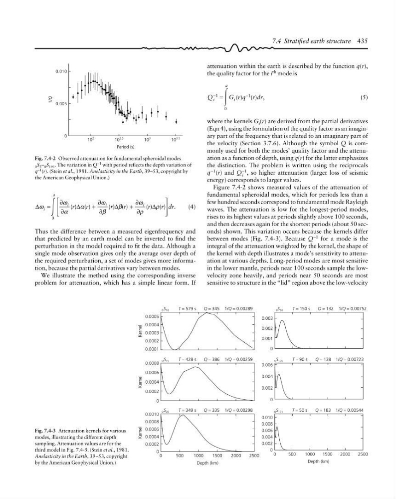
Fig. 7.4-2 Observed attenuation for fundamental spheroidal modes
0 S 2 – 0 S 191 . The variation in Q
−1 with period reflects the depth variation of
q
−1 (r). (Stein et al., 1981. Anelasticity in the Earth, 39–53, copyright by
the American Geophysical Union.)
attenuation within the earth is described by the function q(r),
the quality factor for the i
th mode is
Q i
a
− =
1
0
Ύ
G i (r)q −1 (r)dr,
(5)
where the kernels G i (r) are derived from the partial derivatives
(Eqn 4), using the formulation of the quality factor as an imaginary part of the frequency that is related to an imaginary part of
the velocity (Section 3.7.6). Although the symbol Q is commonly used for both the modes’ quality factor and the attenuation as a function of depth, using q(r) for the latter emphasizes
the distinction. The problem is written using the reciprocals
q −1 (r) and Q i
−1 , so higher attenuation (larger loss of seismic
energy) corresponds to larger values.
Figure 7.4-2 shows measured values of the attenuation of
fundamental spheroidal modes, which for periods less than a
few hundred seconds correspond to fundamental mode Rayleigh
waves. The attenuation is low for the longest-period modes,
rises to its highest values at periods slightly above 100 seconds,
and then decreases again for the shortest periods (about 50 seconds) shown. This variation occurs because the kernels differ
between modes (Fig. 7.4-3). Because Q −1 for a mode is the
integral of the attenuation weighted by the kernel, the shape of
the kernel with depth illustrates a mode’s sensitivity to attenuation at various depths. Long-period modes are most sensitive
in the lower mantle, periods near 100 seconds sample the lowvelocity zone heavily, and periods near 50 seconds are most
sensitive to structure in the “lid” region above the low-velocity
Kernel
0.0005
0.0004
0.0003
0.0002
0.0001
0 S 10
T = 579 s
Q = 345 1/Q = 0.00289
Kernel
0.0008
0.0006
0.0004
0.0002
0
0 S 15
T = 428 s
Q = 386 1/Q = 0.00259
Kernel
0.0010
0.0008
0.0006
0.0004
0.0002
0
0 S 20
T = 349 s
Q = 335 1/Q = 0.00298
0.003
0.002
0.001
0
0 S 60
T = 150 s
Q = 132 1/Q = 0.00752
0
500
1000
1500
2000
2500
Depth (km)
0.006
0.004
0.002
0
0 S 105
T = 90 s
Q = 138 1/Q = 0.00723
0.010
0.008
0.006
0.004
0.002
0
0 S 191
T = 50 s
Q = 183 1/Q = 0.00544
500
1000
1500
2000
2500
Depth (km)
0
∆
∆
∆
∆
ω
ω
α
α
ω
β
β
ω
ρ
ρ
i
a
i
i
i
r
r
r
r
r
r dr
=
+
+
⎡
⎣
⎢
⎢
⎤
⎦
⎥
⎥
( ) ( )
( ) ( )
( ) ( ) .
Ύ
0
∂
∂
∂
∂
∂
∂
(4)
Thus the difference between a measured eigenfrequency and
that predicted by an earth model can be inverted to find the
perturbation in the model required to fit the data. Although a
single mode observation gives only the average over depth of
the required perturbation, a set of modes gives more information, because the partial derivatives vary between modes.
We illustrate the method using the corresponding inverse
problem for attenuation, which has a simple linear form. If
7.4 Stratified earth structure 435
Fig. 7.4-3 Attenuation kernels for various
modes, illustrating the different depth
sampling. Attenuation values are for the
third model in Fig. 7.4-5. (Stein et al., 1981.
Anelasticity in the Earth, 39–53, copyright
by the American Geophysical Union.)
0.010
0.005
0
10
2
10
2.5
10
3
10
3.5
Period (s)
Fig. 7.4-2 Observed attenuation for fundamental spheroidal modes
0 S 2 – 0 S 191 . The variation in Q
−1 with period reflects the depth variation of
q
−1 (r). (Stein et al., 1981. Anelasticity in the Earth, 39–53, copyright by
the American Geophysical Union.)
attenuation within the earth is described by the function q(r),
the quality factor for the i
th mode is
Q i
a
− =
1
0
Ύ
G i (r)q −1 (r)dr,
(5)
where the kernels G i (r) are derived from the partial derivatives
(Eqn 4), using the formulation of the quality factor as an imaginary part of the frequency that is related to an imaginary part of
the velocity (Section 3.7.6). Although the symbol Q is commonly used for both the modes’ quality factor and the attenuation as a function of depth, using q(r) for the latter emphasizes
the distinction. The problem is written using the reciprocals
q −1 (r) and Q i
−1 , so higher attenuation (larger loss of seismic
energy) corresponds to larger values.
Figure 7.4-2 shows measured values of the attenuation of
fundamental spheroidal modes, which for periods less than a
few hundred seconds correspond to fundamental mode Rayleigh
waves. The attenuation is low for the longest-period modes,
rises to its highest values at periods slightly above 100 seconds,
and then decreases again for the shortest periods (about 50 seconds) shown. This variation occurs because the kernels differ
between modes (Fig. 7.4-3). Because Q −1 for a mode is the
integral of the attenuation weighted by the kernel, the shape of
the kernel with depth illustrates a mode’s sensitivity to attenuation at various depths. Long-period modes are most sensitive
in the lower mantle, periods near 100 seconds sample the lowvelocity zone heavily, and periods near 50 seconds are most
sensitive to structure in the “lid” region above the low-velocity
Kernel
0.0005
0.0004
0.0003
0.0002
0.0001
0 S 10
T = 579 s
Q = 345 1/Q = 0.00289
Kernel
0.0008
0.0006
0.0004
0.0002
0
0 S 15
T = 428 s
Q = 386 1/Q = 0.00259
Kernel
0.0010
0.0008
0.0006
0.0004
0.0002
0
0 S 20
T = 349 s
Q = 335 1/Q = 0.00298
0.003
0.002
0.001
0
0 S 60
T = 150 s
Q = 132 1/Q = 0.00752
0
500
1000
1500
2000
2500
Depth (km)
0.006
0.004
0.002
0
0 S 105
T = 90 s
Q = 138 1/Q = 0.00723
0.010
0.008
0.006
0.004
0.002
0
0 S 191
T = 50 s
Q = 183 1/Q = 0.00544
500
1000
1500
2000
2500
Depth (km)
0
∆
∆
∆
∆
ω
ω
α
α
ω
β
β
ω
ρ
ρ
i
a
i
i
i
r
r
r
r
r
r dr
=
+
+
⎡
⎣
⎢
⎢
⎤
⎦
⎥
⎥
( ) ( )
( ) ( )
( ) ( ) .
Ύ
0
∂
∂
∂
∂
∂
∂
(4)
Thus the difference between a measured eigenfrequency and
that predicted by an earth model can be inverted to find the
perturbation in the model required to fit the data. Although a
single mode observation gives only the average over depth of
the required perturbation, a set of modes gives more information, because the partial derivatives vary between modes.
We illustrate the method using the corresponding inverse
problem for attenuation, which has a simple linear form. If
7.4 Stratified earth structure 435
Fig. 7.4-3 Attenuation kernels for various
modes, illustrating the different depth
sampling. Attenuation values are for the
third model in Fig. 7.4-5. (Stein et al., 1981.
Anelasticity in the Earth, 39–53, copyright
by the American Geophysical Union.)