

434 Inverse Problems
+1.5%
−1.5%
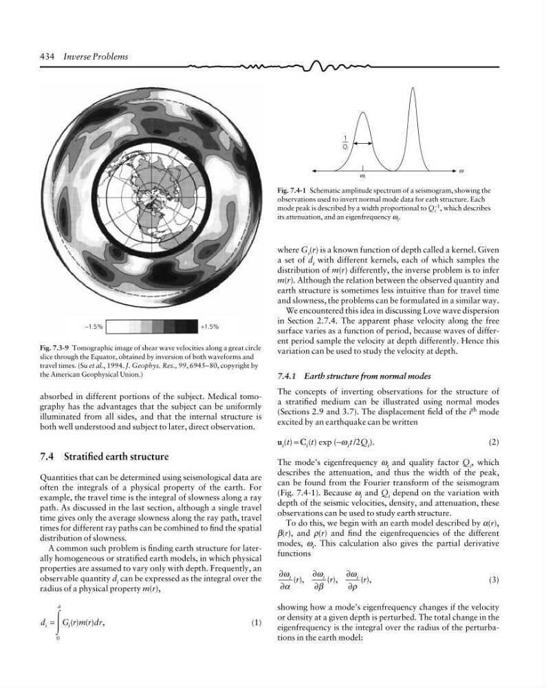
Fig. 7.3-9 Tomographic image of shear wave velocities along a great circle
slice through the Equator, obtained by inversion of both waveforms and
travel times. (Su et al., 1994. J. Geophys. Res., 99, 6945–80, copyright by
the American Geophysical Union.)
absorbed in different portions of the subject. Medical tomography has the advantages that the subject can be uniformly
illuminated from all sides, and that the internal structure is
both well understood and subject to later, direct observation.
7.4 Stratified earth structure
Quantities that can be determined using seismological data are
often the integrals of a physical property of the earth. For
example, the travel time is the integral of slowness along a ray
path. As discussed in the last section, although a single travel
time gives only the average slowness along the ray path, travel
times for different ray paths can be combined to find the spatial
distribution of slowness.
A common such problem is finding earth structure for laterally homogeneous or stratified earth models, in which physical
properties are assumed to vary only with depth. Frequently, an
observable quantity d i can be expressed as the integral over the
radius of a physical property m(r),
d
G r m r dr
i
a
i
=
( ) ( ) ,
Ύ
0
(1)
ω i
ω
ω
1
Q i
Fig. 7.4-1 Schematic amplitude spectrum of a seismogram, showing the
observations used to invert normal mode data for eath structure. Each
mode peak is described by a width proportional to Q i
−1 , which describes
its attenuation, and an eigenfrequency ω i .
where G i (r) is a known function of depth called a kernel. Given
a set of d i with different kernels, each of which samples the
distribution of m(r) differently, the inverse problem is to infer
m(r). Although the relation between the observed quantity and
earth structure is sometimes less intuitive than for travel time
and slowness, the problems can be formulated in a similar way.
We encountered this idea in discussing Love wave dispersion
in Section 2.7.4. The apparent phase velocity along the free
surface varies as a function of period, because waves of different period sample the velocity at depth differently. Hence this
variation can be used to study the velocity at depth.
7.4.1 Earth structure from normal modes
The concepts of inverting observations for the structure of
a stratified medium can be illustrated using normal modes
(Sections 2.9 and 3.7). The displacement field of the i th mode
excited by an earthquake can be written
u i (t) = C i (t) exp (−ω i t /2Q i ).
(2)
The mode’s eigenfrequency ω i and quality factor Q i , which
describes the attenuation, and thus the width of the peak,
can be found from the Fourier transform of the seismogram
(Fig. 7.4-1). Because ω i and Q i depend on the variation with
depth of the seismic velocities, density, and attenuation, these
observations can be used to study earth structure.
To do this, we begin with an earth model described by α(r),
β(r), and ρ(r) and find the eigenfrequencies of the different
modes, ω i . This calculation also gives the partial derivative
functions
∂
∂
∂
∂
∂
∂
ω
α
ω
β
ω
ρ
i
i
i
r
r
r
( ),
( ),
( ),
(3)
showing how a mode’s eigenfrequency changes if the velocity
or density at a given depth is perturbed. The total change in the
eigenfrequency is the integral over the radius of the perturbations in the earth model:
+1.5%
−1.5%
Fig. 7.3-9 Tomographic image of shear wave velocities along a great circle
slice through the Equator, obtained by inversion of both waveforms and
travel times. (Su et al., 1994. J. Geophys. Res., 99, 6945–80, copyright by
the American Geophysical Union.)
absorbed in different portions of the subject. Medical tomography has the advantages that the subject can be uniformly
illuminated from all sides, and that the internal structure is
both well understood and subject to later, direct observation.
7.4 Stratified earth structure
Quantities that can be determined using seismological data are
often the integrals of a physical property of the earth. For
example, the travel time is the integral of slowness along a ray
path. As discussed in the last section, although a single travel
time gives only the average slowness along the ray path, travel
times for different ray paths can be combined to find the spatial
distribution of slowness.
A common such problem is finding earth structure for laterally homogeneous or stratified earth models, in which physical
properties are assumed to vary only with depth. Frequently, an
observable quantity d i can be expressed as the integral over the
radius of a physical property m(r),
d
G r m r dr
i
a
i
=
( ) ( ) ,
Ύ
0
(1)
ω i
ω
ω
1
Q i
Fig. 7.4-1 Schematic amplitude spectrum of a seismogram, showing the
observations used to invert normal mode data for eath structure. Each
mode peak is described by a width proportional to Q i
−1 , which describes
its attenuation, and an eigenfrequency ω i .
where G i (r) is a known function of depth called a kernel. Given
a set of d i with different kernels, each of which samples the
distribution of m(r) differently, the inverse problem is to infer
m(r). Although the relation between the observed quantity and
earth structure is sometimes less intuitive than for travel time
and slowness, the problems can be formulated in a similar way.
We encountered this idea in discussing Love wave dispersion
in Section 2.7.4. The apparent phase velocity along the free
surface varies as a function of period, because waves of different period sample the velocity at depth differently. Hence this
variation can be used to study the velocity at depth.
7.4.1 Earth structure from normal modes
The concepts of inverting observations for the structure of
a stratified medium can be illustrated using normal modes
(Sections 2.9 and 3.7). The displacement field of the i th mode
excited by an earthquake can be written
u i (t) = C i (t) exp (−ω i t /2Q i ).
(2)
The mode’s eigenfrequency ω i and quality factor Q i , which
describes the attenuation, and thus the width of the peak,
can be found from the Fourier transform of the seismogram
(Fig. 7.4-1). Because ω i and Q i depend on the variation with
depth of the seismic velocities, density, and attenuation, these
observations can be used to study earth structure.
To do this, we begin with an earth model described by α(r),
β(r), and ρ(r) and find the eigenfrequencies of the different
modes, ω i . This calculation also gives the partial derivative
functions
∂
∂
∂
∂
∂
∂
ω
α
ω
β
ω
ρ
i
i
i
r
r
r
( ),
( ),
( ),
(3)
showing how a mode’s eigenfrequency changes if the velocity
or density at a given depth is perturbed. The total change in the
eigenfrequency is the integral over the radius of the perturbations in the earth model: