

age range, and then infer the variation in the medium velocity
with depth from the dispersion curve giving the variation in
apparent velocity as a function of frequency. Hence this is
tomography in the lateral direction, and dispersion analysis
vertically. We will see in the next section that dispersion analysis is an example of methods that infer earth structure using
functions that sample the structure at depth in different ways.
Tomographic methods can be used for waveforms as well as
travel times. As noted earlier a for example, in Fig. 3.7-7 a
waveforms sample earth structure over broader regions than
travel times, which, in the limit, correspond to sampling along
narrow geometric rays. Figure 7.3-9 shows some results
from global tomography in which velocity perturbations were
inferred by fitting both waveforms from 27,000 long-period
seismograms and 14,000 travel times. The seismograms include
body wave records (from the P or PKP arrival to the start of the
surface waves) and “mantle wave” records, which are low-pass
filtered seismograms about 4.5 hours in length. The travel time
data include both absolute shear wave arrival times and differential (SS–S and ScS–S) times. Rather than inverting for the
velocity perturbations in blocks, the velocity perturbation was
described by a series of orthogonal functions, and the inversion
was for the coefficients of the functions. The lateral structure
was described by spherical harmonics (Section 2.9.3), and the
vertical structure was modeled using Chebyshev polynomials.
In addition, we saw in Section 3.7 that amplitude tomography can infer attenuation variations along the ray paths.
Amplitude tomography is similar to medical tomography, 4
in which the image indicates the degree to which X-rays are
Receivers
150 m
250 m
350 m
150 m
250 m
350 m
Source
175 m
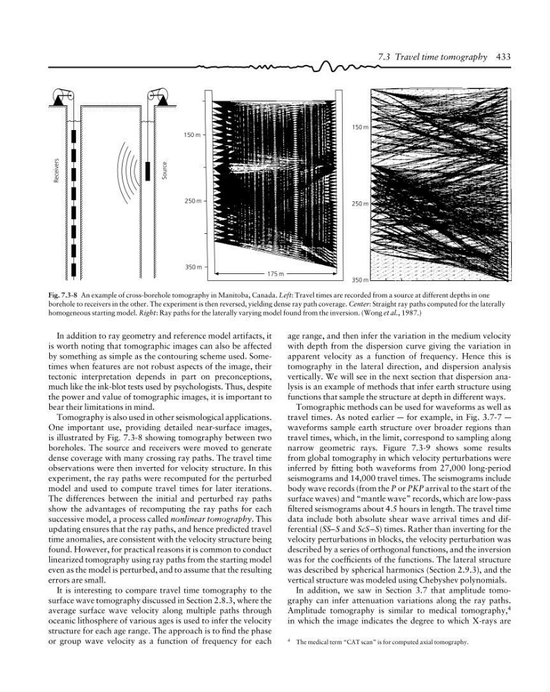
Fig. 7.3-8 An example of cross-borehole tomography in Manitoba, Canada. Left: Travel times are recorded from a source at different depths in one
borehole to receivers in the other. The experiment is then reversed, yielding dense ray path coverage. Center: Straight ray paths computed for the laterally
homogeneous starting model. Right: Ray paths for the laterally varying model found from the inversion. (Wong et al., 1987.)
In addition to ray geometry and reference model artifacts, it
is worth noting that tomographic images can also be affected
by something as simple as the contouring scheme used. Sometimes when features are not robust aspects of the image, their
tectonic interpretation depends in part on preconceptions,
much like the ink-blot tests used by psychologists. Thus, despite
the power and value of tomographic images, it is important to
bear their limitations in mind.
Tomography is also used in other seismological applications.
One important use, providing detailed near-surface images,
is illustrated by Fig. 7.3-8 showing tomography between two
boreholes. The source and receivers were moved to generate
dense coverage with many crossing ray paths. The travel time
observations were then inverted for velocity structure. In this
experiment, the ray paths were recomputed for the perturbed
model and used to compute travel times for later iterations.
The differences between the initial and perturbed ray paths
show the advantages of recomputing the ray paths for each
successive model, a process called nonlinear tomography. This
updating ensures that the ray paths, and hence predicted travel
time anomalies, are consistent with the velocity structure being
found. However, for practical reasons it is common to conduct
linearized tomography using ray paths from the starting model
even as the model is perturbed, and to assume that the resulting
errors are small.
It is interesting to compare travel time tomography to the
surface wave tomography discussed in Section 2.8.3, where the
average surface wave velocity along multiple paths through
oceanic lithosphere of various ages is used to infer the velocity
structure for each age range. The approach is to find the phase
or group wave velocity as a function of frequency for each
4 The medical term “CAT scan” is for computed axial tomography.
7.3 Travel time tomography 433
with depth from the dispersion curve giving the variation in
apparent velocity as a function of frequency. Hence this is
tomography in the lateral direction, and dispersion analysis
vertically. We will see in the next section that dispersion analysis is an example of methods that infer earth structure using
functions that sample the structure at depth in different ways.
Tomographic methods can be used for waveforms as well as
travel times. As noted earlier a for example, in Fig. 3.7-7 a
waveforms sample earth structure over broader regions than
travel times, which, in the limit, correspond to sampling along
narrow geometric rays. Figure 7.3-9 shows some results
from global tomography in which velocity perturbations were
inferred by fitting both waveforms from 27,000 long-period
seismograms and 14,000 travel times. The seismograms include
body wave records (from the P or PKP arrival to the start of the
surface waves) and “mantle wave” records, which are low-pass
filtered seismograms about 4.5 hours in length. The travel time
data include both absolute shear wave arrival times and differential (SS–S and ScS–S) times. Rather than inverting for the
velocity perturbations in blocks, the velocity perturbation was
described by a series of orthogonal functions, and the inversion
was for the coefficients of the functions. The lateral structure
was described by spherical harmonics (Section 2.9.3), and the
vertical structure was modeled using Chebyshev polynomials.
In addition, we saw in Section 3.7 that amplitude tomography can infer attenuation variations along the ray paths.
Amplitude tomography is similar to medical tomography, 4
in which the image indicates the degree to which X-rays are
Receivers
150 m
250 m
350 m
150 m
250 m
350 m
Source
175 m
Fig. 7.3-8 An example of cross-borehole tomography in Manitoba, Canada. Left: Travel times are recorded from a source at different depths in one
borehole to receivers in the other. The experiment is then reversed, yielding dense ray path coverage. Center: Straight ray paths computed for the laterally
homogeneous starting model. Right: Ray paths for the laterally varying model found from the inversion. (Wong et al., 1987.)
In addition to ray geometry and reference model artifacts, it
is worth noting that tomographic images can also be affected
by something as simple as the contouring scheme used. Sometimes when features are not robust aspects of the image, their
tectonic interpretation depends in part on preconceptions,
much like the ink-blot tests used by psychologists. Thus, despite
the power and value of tomographic images, it is important to
bear their limitations in mind.
Tomography is also used in other seismological applications.
One important use, providing detailed near-surface images,
is illustrated by Fig. 7.3-8 showing tomography between two
boreholes. The source and receivers were moved to generate
dense coverage with many crossing ray paths. The travel time
observations were then inverted for velocity structure. In this
experiment, the ray paths were recomputed for the perturbed
model and used to compute travel times for later iterations.
The differences between the initial and perturbed ray paths
show the advantages of recomputing the ray paths for each
successive model, a process called nonlinear tomography. This
updating ensures that the ray paths, and hence predicted travel
time anomalies, are consistent with the velocity structure being
found. However, for practical reasons it is common to conduct
linearized tomography using ray paths from the starting model
even as the model is perturbed, and to assume that the resulting
errors are small.
It is interesting to compare travel time tomography to the
surface wave tomography discussed in Section 2.8.3, where the
average surface wave velocity along multiple paths through
oceanic lithosphere of various ages is used to infer the velocity
structure for each age range. The approach is to find the phase
or group wave velocity as a function of frequency for each
4 The medical term “CAT scan” is for computed axial tomography.
7.3 Travel time tomography 433