

432 Inverse Problems
variations. However, because these variations are with respect
to a starting model, which is usually laterally homogeneous,
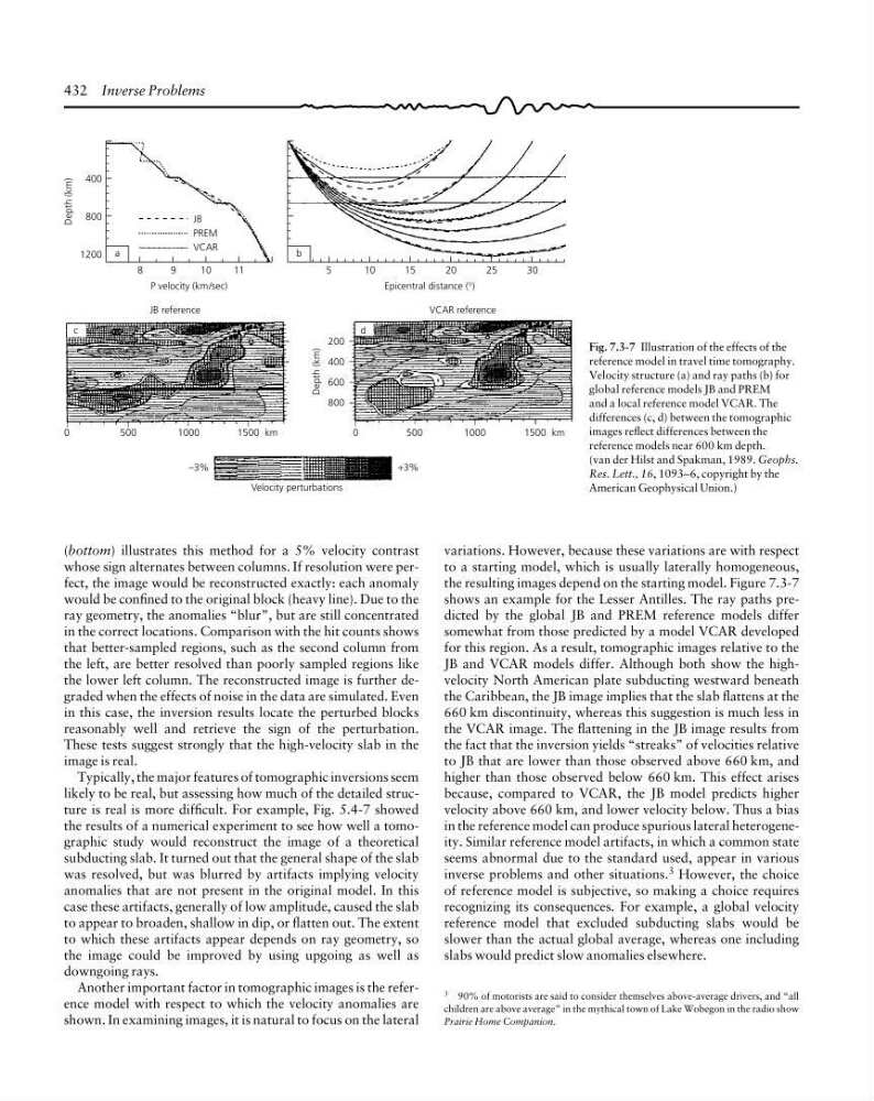
the resulting images depend on the starting model. Figure 7.3-7
shows an example for the Lesser Antilles. The ray paths predicted by the global JB and PREM reference models differ
somewhat from those predicted by a model VCAR developed
for this region. As a result, tomographic images relative to the
JB and VCAR models differ. Although both show the highvelocity North American plate subducting westward beneath
the Caribbean, the JB image implies that the slab flattens at the
660 km discontinuity, whereas this suggestion is much less in
the VCAR image. The flattening in the JB image results from
the fact that the inversion yields “streaks” of velocities relative
to JB that are lower than those observed above 660 km, and
higher than those observed below 660 km. This effect arises
because, compared to VCAR, the JB model predicts higher
velocity above 660 km, and lower velocity below. Thus a bias
in the reference model can produce spurious lateral heterogeneity. Similar reference model artifacts, in which a common state
seems abnormal due to the standard used, appear in various
inverse problems and other situations. 3 However, the choice
of reference model is subjective, so making a choice requires
recognizing its consequences. For example, a global velocity
reference model that excluded subducting slabs would be
slower than the actual global average, whereas one including
slabs would predict slow anomalies elsewhere.
Depth (km)
400
800
1200 a
8
9
10
11
P velocity (km/sec)
b
5
1 0
1 5
2 0
Epicentral distance (°)
25
30
200
400
600
800
Depth (km)
0
500
1000
1500 km
0
500
1000
1500 km
+3%
–3%
Velocity perturbations
JB
PREM
VCAR
JB reference
VCAR reference
c
d
(bottom) illustrates this method for a 5% velocity contrast
whose sign alternates between columns. If resolution were perfect, the image would be reconstructed exactly: each anomaly
would be confined to the original block (heavy line). Due to the
ray geometry, the anomalies “blur”, but are still concentrated
in the correct locations. Comparison with the hit counts shows
that better-sampled regions, such as the second column from
the left, are better resolved than poorly sampled regions like
the lower left column. The reconstructed image is further degraded when the effects of noise in the data are simulated. Even
in this case, the inversion results locate the perturbed blocks
reasonably well and retrieve the sign of the perturbation.
These tests suggest strongly that the high-velocity slab in the
image is real.
Typically, the major features of tomographic inversions seem
likely to be real, but assessing how much of the detailed structure is real is more difficult. For example, Fig. 5.4-7 showed
the results of a numerical experiment to see how well a tomographic study would reconstruct the image of a theoretical
subducting slab. It turned out that the general shape of the slab
was resolved, but was blurred by artifacts implying velocity
anomalies that are not present in the original model. In this
case these artifacts, generally of low amplitude, caused the slab
to appear to broaden, shallow in dip, or flatten out. The extent
to which these artifacts appear depends on ray geometry, so
the image could be improved by using upgoing as well as
downgoing rays.
Another important factor in tomographic images is the reference model with respect to which the velocity anomalies are
shown. In examining images, it is natural to focus on the lateral
3 90% of motorists are said to consider themselves above-average drivers, and “all
children are above average” in the mythical town of Lake Wobegon in the radio show
Prairie Home Companion.
Fig. 7.3-7 Illustration of the effects of the
reference model in travel time tomography.
Velocity structure (a) and ray paths (b) for
global reference models JB and PREM
and a local reference model VCAR. The
differences (c, d) between the tomographic
images reflect differences between the
reference models near 600 km depth.
(van der Hilst and Spakman, 1989. Geophs.
Res. Lett., 16, 1093–6, copyright by the
American Geophysical Union.)
variations. However, because these variations are with respect
to a starting model, which is usually laterally homogeneous,
the resulting images depend on the starting model. Figure 7.3-7
shows an example for the Lesser Antilles. The ray paths predicted by the global JB and PREM reference models differ
somewhat from those predicted by a model VCAR developed
for this region. As a result, tomographic images relative to the
JB and VCAR models differ. Although both show the highvelocity North American plate subducting westward beneath
the Caribbean, the JB image implies that the slab flattens at the
660 km discontinuity, whereas this suggestion is much less in
the VCAR image. The flattening in the JB image results from
the fact that the inversion yields “streaks” of velocities relative
to JB that are lower than those observed above 660 km, and
higher than those observed below 660 km. This effect arises
because, compared to VCAR, the JB model predicts higher
velocity above 660 km, and lower velocity below. Thus a bias
in the reference model can produce spurious lateral heterogeneity. Similar reference model artifacts, in which a common state
seems abnormal due to the standard used, appear in various
inverse problems and other situations. 3 However, the choice
of reference model is subjective, so making a choice requires
recognizing its consequences. For example, a global velocity
reference model that excluded subducting slabs would be
slower than the actual global average, whereas one including
slabs would predict slow anomalies elsewhere.
Depth (km)
400
800
1200 a
8
9
10
11
P velocity (km/sec)
b
5
1 0
1 5
2 0
Epicentral distance (°)
25
30
200
400
600
800
Depth (km)
0
500
1000
1500 km
0
500
1000
1500 km
+3%
–3%
Velocity perturbations
JB
PREM
VCAR
JB reference
VCAR reference
c
d
(bottom) illustrates this method for a 5% velocity contrast
whose sign alternates between columns. If resolution were perfect, the image would be reconstructed exactly: each anomaly
would be confined to the original block (heavy line). Due to the
ray geometry, the anomalies “blur”, but are still concentrated
in the correct locations. Comparison with the hit counts shows
that better-sampled regions, such as the second column from
the left, are better resolved than poorly sampled regions like
the lower left column. The reconstructed image is further degraded when the effects of noise in the data are simulated. Even
in this case, the inversion results locate the perturbed blocks
reasonably well and retrieve the sign of the perturbation.
These tests suggest strongly that the high-velocity slab in the
image is real.
Typically, the major features of tomographic inversions seem
likely to be real, but assessing how much of the detailed structure is real is more difficult. For example, Fig. 5.4-7 showed
the results of a numerical experiment to see how well a tomographic study would reconstruct the image of a theoretical
subducting slab. It turned out that the general shape of the slab
was resolved, but was blurred by artifacts implying velocity
anomalies that are not present in the original model. In this
case these artifacts, generally of low amplitude, caused the slab
to appear to broaden, shallow in dip, or flatten out. The extent
to which these artifacts appear depends on ray geometry, so
the image could be improved by using upgoing as well as
downgoing rays.
Another important factor in tomographic images is the reference model with respect to which the velocity anomalies are
shown. In examining images, it is natural to focus on the lateral
3 90% of motorists are said to consider themselves above-average drivers, and “all
children are above average” in the mythical town of Lake Wobegon in the radio show
Prairie Home Companion.
Fig. 7.3-7 Illustration of the effects of the
reference model in travel time tomography.
Velocity structure (a) and ray paths (b) for
global reference models JB and PREM
and a local reference model VCAR. The
differences (c, d) between the tomographic
images reflect differences between the
reference models near 600 km depth.
(van der Hilst and Spakman, 1989. Geophs.
Res. Lett., 16, 1093–6, copyright by the
American Geophysical Union.)