

Depth (km)
200
400
600
500
1000
Distance (km)
–3%
+3%
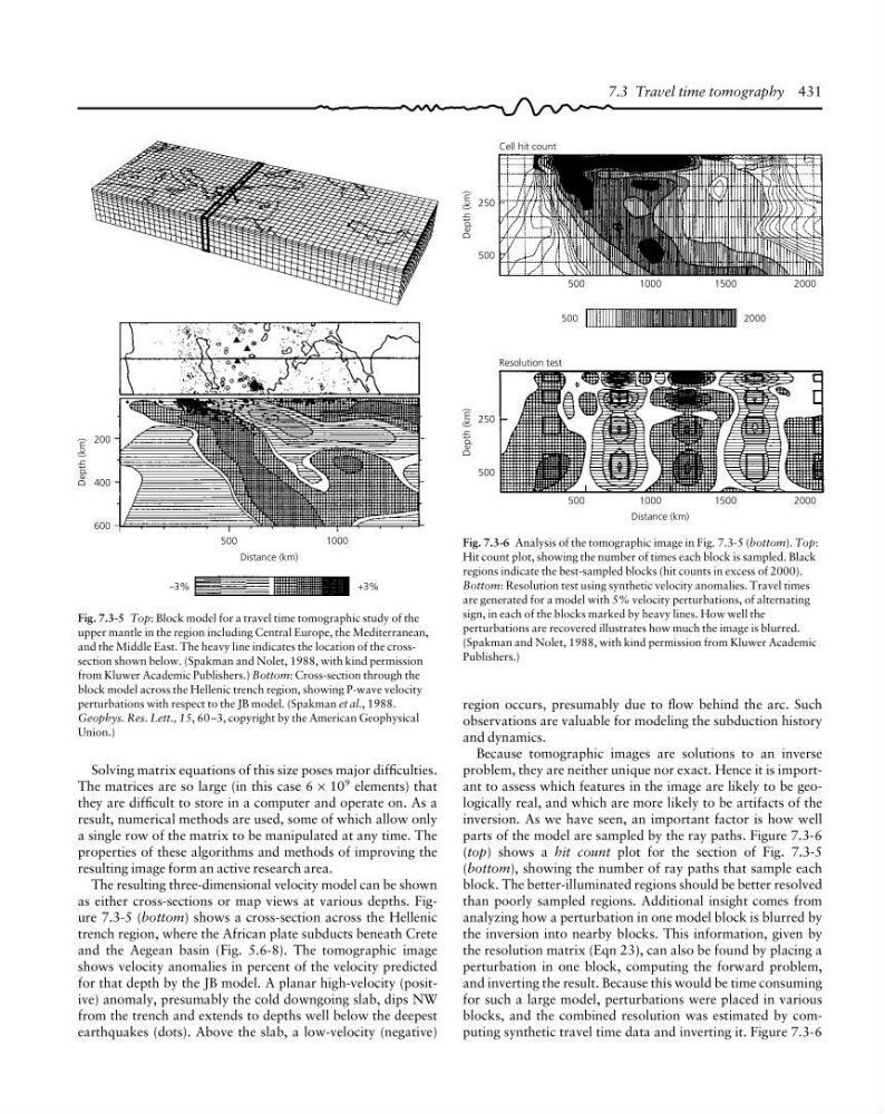
Fig. 7.3-5 Top: Block model for a travel time tomographic study of the
upper mantle in the region including Central Europe, the Mediterranean,
and the Middle East. The heavy line indicates the location of the crosssection shown below. (Spakman and Nolet, 1988, with kind permission
from Kluwer Academic Publishers.) Bottom: Cross-section through the
block model across the Hellenic trench region, showing P-wave velocity
perturbations with respect to the JB model. (Spakman et al., 1988.
Geophys. Res. Lett., 15, 60–3, copyright by the American Geophysical
Union.)
Depth (km)
250
500
500
1000
1500
2000
500
2000
Cell hit count
Resolution test
Depth (km)
250
500
500
1000
1500
2000
Distance (km)
Fig. 7.3-6 Analysis of the tomographic image in Fig. 7.3-5 (bottom). Top:
Hit count plot, showing the number of times each block is sampled. Black
regions indicate the best-sampled blocks (hit counts in excess of 2000).
Bottom: Resolution test using synthetic velocity anomalies. Travel times
are generated for a model with 5% velocity perturbations, of alternating
sign, in each of the blocks marked by heavy lines. How well the
perturbations are recovered illustrates how much the image is blurred.
(Spakman and Nolet, 1988, with kind permission from Kluwer Academic
Publishers.)
region occurs, presumably due to flow behind the arc. Such
observations are valuable for modeling the subduction history
and dynamics.
Because tomographic images are solutions to an inverse
problem, they are neither unique nor exact. Hence it is important to assess which features in the image are likely to be geologically real, and which are more likely to be artifacts of the
inversion. As we have seen, an important factor is how well
parts of the model are sampled by the ray paths. Figure 7.3-6
(top) shows a hit count plot for the section of Fig. 7.3-5
(bottom), showing the number of ray paths that sample each
block. The better-illuminated regions should be better resolved
than poorly sampled regions. Additional insight comes from
analyzing how a perturbation in one model block is blurred by
the inversion into nearby blocks. This information, given by
the resolution matrix (Eqn 23), can also be found by placing a
perturbation in one block, computing the forward problem,
and inverting the result. Because this would be time consuming
for such a large model, perturbations were placed in various
blocks, and the combined resolution was estimated by computing synthetic travel time data and inverting it. Figure 7.3-6
7.3 Travel time tomography 431
Solving matrix equations of this size poses major difficulties.
The matrices are so large (in this case 6 × 10 9 elements) that
they are difficult to store in a computer and operate on. As a
result, numerical methods are used, some of which allow only
a single row of the matrix to be manipulated at any time. The
properties of these algorithms and methods of improving the
resulting image form an active research area.
The resulting three-dimensional velocity model can be shown
as either cross-sections or map views at various depths. Figure 7.3-5 (bottom) shows a cross-section across the Hellenic
trench region, where the African plate subducts beneath Crete
and the Aegean basin (Fig. 5.6-8). The tomographic image
shows velocity anomalies in percent of the velocity predicted
for that depth by the JB model. A planar high-velocity (positive) anomaly, presumably the cold downgoing slab, dips NW
from the trench and extends to depths well below the deepest
earthquakes (dots). Above the slab, a low-velocity (negative)
200
400
600
500
1000
Distance (km)
–3%
+3%
Fig. 7.3-5 Top: Block model for a travel time tomographic study of the
upper mantle in the region including Central Europe, the Mediterranean,
and the Middle East. The heavy line indicates the location of the crosssection shown below. (Spakman and Nolet, 1988, with kind permission
from Kluwer Academic Publishers.) Bottom: Cross-section through the
block model across the Hellenic trench region, showing P-wave velocity
perturbations with respect to the JB model. (Spakman et al., 1988.
Geophys. Res. Lett., 15, 60–3, copyright by the American Geophysical
Union.)
Depth (km)
250
500
500
1000
1500
2000
500
2000
Cell hit count
Resolution test
Depth (km)
250
500
500
1000
1500
2000
Distance (km)
Fig. 7.3-6 Analysis of the tomographic image in Fig. 7.3-5 (bottom). Top:
Hit count plot, showing the number of times each block is sampled. Black
regions indicate the best-sampled blocks (hit counts in excess of 2000).
Bottom: Resolution test using synthetic velocity anomalies. Travel times
are generated for a model with 5% velocity perturbations, of alternating
sign, in each of the blocks marked by heavy lines. How well the
perturbations are recovered illustrates how much the image is blurred.
(Spakman and Nolet, 1988, with kind permission from Kluwer Academic
Publishers.)
region occurs, presumably due to flow behind the arc. Such
observations are valuable for modeling the subduction history
and dynamics.
Because tomographic images are solutions to an inverse
problem, they are neither unique nor exact. Hence it is important to assess which features in the image are likely to be geologically real, and which are more likely to be artifacts of the
inversion. As we have seen, an important factor is how well
parts of the model are sampled by the ray paths. Figure 7.3-6
(top) shows a hit count plot for the section of Fig. 7.3-5
(bottom), showing the number of ray paths that sample each
block. The better-illuminated regions should be better resolved
than poorly sampled regions. Additional insight comes from
analyzing how a perturbation in one model block is blurred by
the inversion into nearby blocks. This information, given by
the resolution matrix (Eqn 23), can also be found by placing a
perturbation in one block, computing the forward problem,
and inverting the result. Because this would be time consuming
for such a large model, perturbations were placed in various
blocks, and the combined resolution was estimated by computing synthetic travel time data and inverting it. Figure 7.3-6
7.3 Travel time tomography 431
Solving matrix equations of this size poses major difficulties.
The matrices are so large (in this case 6 × 10 9 elements) that
they are difficult to store in a computer and operate on. As a
result, numerical methods are used, some of which allow only
a single row of the matrix to be manipulated at any time. The
properties of these algorithms and methods of improving the
resulting image form an active research area.
The resulting three-dimensional velocity model can be shown
as either cross-sections or map views at various depths. Figure 7.3-5 (bottom) shows a cross-section across the Hellenic
trench region, where the African plate subducts beneath Crete
and the Aegean basin (Fig. 5.6-8). The tomographic image
shows velocity anomalies in percent of the velocity predicted
for that depth by the JB model. A planar high-velocity (positive) anomaly, presumably the cold downgoing slab, dips NW
from the trench and extends to depths well below the deepest
earthquakes (dots). Above the slab, a low-velocity (negative)