

428 Inverse Problems
0
0
1
0
0
0
1
0
0
0
1
0
0.25
0.25
0.75
–0.25
True structure
Resolved structure
V matrices their form, controls the resolution. Note that in the
first example, in which all six ray paths are used, Eqn 9 shows
that the model from the inversion was the true model. In this
case the resolution matrix is the identity matrix.
To see how the lack of resolution in the four-ray case arises,
consider what would occur if G T G had no zero eigenvalues and
could be inverted. Then, by Eqns 21 and 22, the model derived
from the data would be
m p = VΛ p
−1 U T
p d,
(27)
because V p = V. The model is thus a linear combination of
the columns of V, or the eigenvectors of G T G. Because there
are r (in this case four) linearly independent eigenvectors, and
the model vector has r elements, the eigenvectors span the
r-dimensional model space. Thus any vector in the model space
is a possible model.
If instead, as in this case, some of the eigenvalues are zero,
the eigenvectors associated with them are excluded from the V p
matrix. The model
m p = V p Λ p
−1 U T
p d
(28)
is then a linear combination of only the columns of V p , the
eigenvectors associated with the nonzero eigenvalues. In this
case, there are r − p (here three) rather than r linearly independent eigenvectors. Hence not all possible vectors in the model
space can be constructed. The model resulting from the inversion contains no linear combinations of the eigenvectors associated with the zero eigenvalues.
To illustrate this idea, consider the four-ray case where the
eigenvector associated with the zero eigenvalue is (from Eqn 25)
v = (0.5, 0.5, −0.5, −0.5) T .
(29)
This vector corresponds to equal slowness perturbations in
blocks 1 and 2 and equal perturbations of opposite sign in
blocks 3 and 4. Physically, this means changing the slowness
everywhere in the upper layer by some amount, and making the
opposite change in the lower layer. Because all four teleseismic
rays have equal path lengths in the upper and lower layers,
their travel times are unaffected, so travel time data cannot
resolve any such change.
Another way to see this is to consider Eqn 7 and note that if
v is an eigenvector whose eigenvalue is zero,
(G T G)v = 0,
(30)
so that even if the model contains a linear combination of such
eigenvectors, they have no effect on the problem. The zero
eigenvectors thus limit the resolution of the model. Because any
linear combination of these eigenvectors has no effect, the
model resulting from the inversion is not unique. It is possible
to prove that the generalized inverse G −p finds a “best” model
with no contribution from these eigenvectors. Mathematically,
the resulting model is restricted to the V p space and has no components in the V 0 space. As a result, this model is the minimum
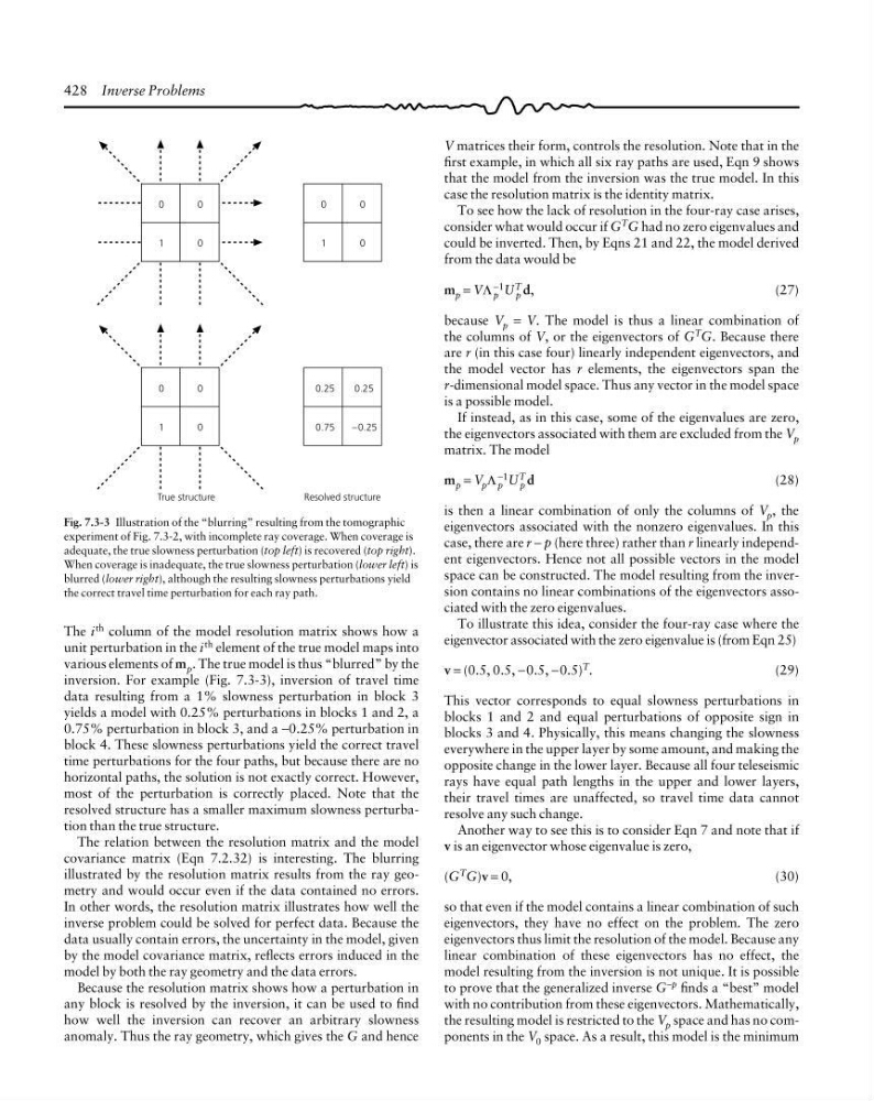
Fig. 7.3-3 Illustration of the “blurring” resulting from the tomographic
experiment of Fig. 7.3-2, with incomplete ray coverage. When coverage is
adequate, the true slowness perturbation (top left) is recovered (top right).
When coverage is inadequate, the true slowness perturbation (lower left) is
blurred (lower right), although the resulting slowness perturbations yield
the correct travel time perturbation for each ray path.
The i
th column of the model resolution matrix shows how a
unit perturbation in the i th element of the true model maps into
various elements of m p . The true model is thus “blurred” by the
inversion. For example (Fig. 7.3-3), inversion of travel time
data resulting from a 1% slowness perturbation in block 3
yields a model with 0.25% perturbations in blocks 1 and 2, a
0.75% perturbation in block 3, and a −0.25% perturbation in
block 4. These slowness perturbations yield the correct travel
time perturbations for the four paths, but because there are no
horizontal paths, the solution is not exactly correct. However,
most of the perturbation is correctly placed. Note that the
resolved structure has a smaller maximum slowness perturbation than the true structure.
The relation between the resolution matrix and the model
covariance matrix (Eqn 7.2.32) is interesting. The blurring
illustrated by the resolution matrix results from the ray geometry and would occur even if the data contained no errors.
In other words, the resolution matrix illustrates how well the
inverse problem could be solved for perfect data. Because the
data usually contain errors, the uncertainty in the model, given
by the model covariance matrix, reflects errors induced in the
model by both the ray geometry and the data errors.
Because the resolution matrix shows how a perturbation in
any block is resolved by the inversion, it can be used to find
how well the inversion can recover an arbitrary slowness
anomaly. Thus the ray geometry, which gives the G and hence
0
0
1
0
0
0
1
0
0
0
1
0
0.25
0.25
0.75
–0.25
True structure
Resolved structure
V matrices their form, controls the resolution. Note that in the
first example, in which all six ray paths are used, Eqn 9 shows
that the model from the inversion was the true model. In this
case the resolution matrix is the identity matrix.
To see how the lack of resolution in the four-ray case arises,
consider what would occur if G T G had no zero eigenvalues and
could be inverted. Then, by Eqns 21 and 22, the model derived
from the data would be
m p = VΛ p
−1 U T
p d,
(27)
because V p = V. The model is thus a linear combination of
the columns of V, or the eigenvectors of G T G. Because there
are r (in this case four) linearly independent eigenvectors, and
the model vector has r elements, the eigenvectors span the
r-dimensional model space. Thus any vector in the model space
is a possible model.
If instead, as in this case, some of the eigenvalues are zero,
the eigenvectors associated with them are excluded from the V p
matrix. The model
m p = V p Λ p
−1 U T
p d
(28)
is then a linear combination of only the columns of V p , the
eigenvectors associated with the nonzero eigenvalues. In this
case, there are r − p (here three) rather than r linearly independent eigenvectors. Hence not all possible vectors in the model
space can be constructed. The model resulting from the inversion contains no linear combinations of the eigenvectors associated with the zero eigenvalues.
To illustrate this idea, consider the four-ray case where the
eigenvector associated with the zero eigenvalue is (from Eqn 25)
v = (0.5, 0.5, −0.5, −0.5) T .
(29)
This vector corresponds to equal slowness perturbations in
blocks 1 and 2 and equal perturbations of opposite sign in
blocks 3 and 4. Physically, this means changing the slowness
everywhere in the upper layer by some amount, and making the
opposite change in the lower layer. Because all four teleseismic
rays have equal path lengths in the upper and lower layers,
their travel times are unaffected, so travel time data cannot
resolve any such change.
Another way to see this is to consider Eqn 7 and note that if
v is an eigenvector whose eigenvalue is zero,
(G T G)v = 0,
(30)
so that even if the model contains a linear combination of such
eigenvectors, they have no effect on the problem. The zero
eigenvectors thus limit the resolution of the model. Because any
linear combination of these eigenvectors has no effect, the
model resulting from the inversion is not unique. It is possible
to prove that the generalized inverse G −p finds a “best” model
with no contribution from these eigenvectors. Mathematically,
the resulting model is restricted to the V p space and has no components in the V 0 space. As a result, this model is the minimum
Fig. 7.3-3 Illustration of the “blurring” resulting from the tomographic
experiment of Fig. 7.3-2, with incomplete ray coverage. When coverage is
adequate, the true slowness perturbation (top left) is recovered (top right).
When coverage is inadequate, the true slowness perturbation (lower left) is
blurred (lower right), although the resulting slowness perturbations yield
the correct travel time perturbation for each ray path.
The i
th column of the model resolution matrix shows how a
unit perturbation in the i th element of the true model maps into
various elements of m p . The true model is thus “blurred” by the
inversion. For example (Fig. 7.3-3), inversion of travel time
data resulting from a 1% slowness perturbation in block 3
yields a model with 0.25% perturbations in blocks 1 and 2, a
0.75% perturbation in block 3, and a −0.25% perturbation in
block 4. These slowness perturbations yield the correct travel
time perturbations for the four paths, but because there are no
horizontal paths, the solution is not exactly correct. However,
most of the perturbation is correctly placed. Note that the
resolved structure has a smaller maximum slowness perturbation than the true structure.
The relation between the resolution matrix and the model
covariance matrix (Eqn 7.2.32) is interesting. The blurring
illustrated by the resolution matrix results from the ray geometry and would occur even if the data contained no errors.
In other words, the resolution matrix illustrates how well the
inverse problem could be solved for perfect data. Because the
data usually contain errors, the uncertainty in the model, given
by the model covariance matrix, reflects errors induced in the
model by both the ray geometry and the data errors.
Because the resolution matrix shows how a perturbation in
any block is resolved by the inversion, it can be used to find
how well the inversion can recover an arbitrary slowness
anomaly. Thus the ray geometry, which gives the G and hence