

possible solution consistent with the data. In this application,
the minimum model gives the least lateral perturbation in
slowness consistent with the travel time data. Philosophically,
this is an attractive approach.
The six-ray case, by contrast, had no zero eigenvalues.
Because one ray traveled only in the upper layer and another
traveled only in the lower layer, a change in the slowness in
either layer would affect the travel times. This ray geometry
avoids the ambiguity of the four-ray case, so the model is fully
resolved. There is no V 0 space, so V = V p , G T G can be inverted,
and the solution is found using the generalized inverse G −g
(Eqn 8). To see how this is related to the generalized inverse
G −p , we use the Lanczos decomposition (Eqn 20) to expand G:
G T G = (VΛ p U T
p )(U p Λ p V T ) = VΛ 2
p V T ,
(31)
(G T G) −1 = VΛ p
−2 V T ,
(32)
where the matrix products Λ 2
p = Λ p Λ p and Λ p
−2 = Λ p
−1 Λ p
−1 . Thus,
if G T G can be inverted, the generalized inverse
G −g = (G T G) −1 G T = (VΛ p
−2 V T )(VΛ p U T
p ) = VΛ p
−1 U T
p = G −p . (33)
Hence G −p is the general form of the generalized inverse, and
G −g is the special form that applies if G T G can be inverted. The
later form, G −g , is easier to compute because it does not require
the eigenvector decomposition. Fortunately, it can often be
used in applications such as earthquake location.
The eigenvector decomposition also divides the data space
into two portions, U p and U 0 , reflecting the nonzero and zero
eigenvalues. Data vectors in the U 0 space, linear combinations
of the eigenvectors whose eigenvalues are zero, cannot be generated by the operator G for any model. For example, in the
six-ray case there cannot be six linearly independent observations because the model has only four parameters. Thus two of
the six eigenvectors of the 6 × 6 matrix GG T must have zero
eigenvalues. These eigenvectors represent travel time observations that should be impossible, given the geometry of the
experiment. If the data contained some linear combinations
of these eigenvectors, perhaps due to noise in the data, the
inversion process could never generate a model capable of
matching them.
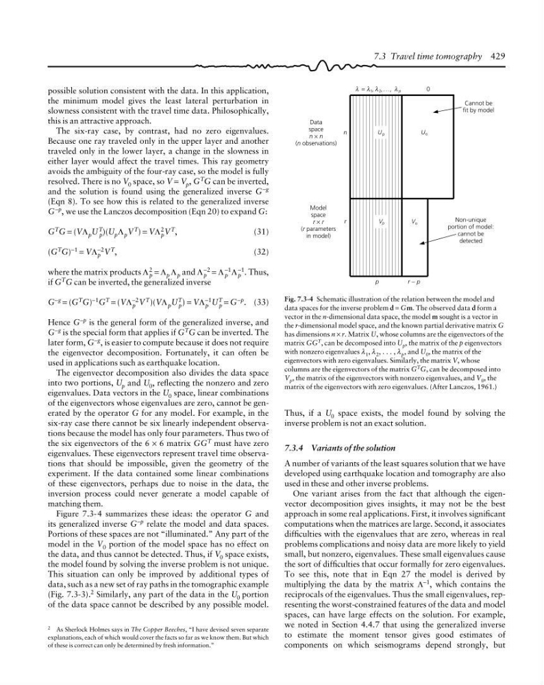
Figure 7.3-4 summarizes these ideas: the operator G and
its generalized inverse G −p relate the model and data spaces.
Portions of these spaces are not “illuminated.” Any part of the
model in the V 0 portion of the model space has no effect on
the data, and thus cannot be detected. Thus, if V 0 space exists,
the model found by solving the inverse problem is not unique.
This situation can only be improved by additional types of
data, such as a new set of ray paths in the tomographic example
(Fig. 7.3-3). 2 Similarly, any part of the data in the U 0 portion
of the data space cannot be described by any possible model.
7.3 Travel time tomography 429
2 As Sherlock Holmes says in The Copper Beeches, “I have devised seven separate
explanations, each of which would cover the facts so far as we know them. But which
of these is correct can only be determined by fresh information.”
n
U
U
r
V
V
o
o
0
λ = λ , λ ,..., λ
1
2
p
p
r − p
Data
space
n × n
(n observations)
Model
space
r × r
(r parameters
in model)
Cannot be
fit by model
Non-unique
portion of model:
cannot be
detected
p
p
Fig. 7.3-4 Schematic illustration of the relation between the model and
data spaces for the inverse problem d = Gm. The observed data d form a
vector in the n-dimensional data space, the model m sought is a vector in
the r-dimensional model space, and the known partial derivative matrix G
has dimensions n × r. Matrix U, whose columns are the eigenvectors of the
matrix GG
T , can be decomposed into U p , the matrix of the p eigenvectors
with nonzero eigenvalues λ 1 , λ 2 , . . . , λ p , and U 0 , the matrix of the
eigenvectors with zero eigenvalues. Similarly, the matrix V, whose
columns are the eigenvectors of the matrix G T G, can be decomposed into
V p , the matrix of the eigenvectors with nonzero eigenvalues, and V 0 , the
matrix of the eigenvectors with zero eigenvalues. (After Lanczos, 1961.)
Thus, if a U 0 space exists, the model found by solving the
inverse problem is not an exact solution.
7.3.4 Variants of the solution
A number of variants of the least squares solution that we have
developed using earthquake location and tomography are also
used in these and other inverse problems.
One variant arises from the fact that although the eigenvector decomposition gives insights, it may not be the best
approach in some real applications. First, it involves significant
computations when the matrices are large. Second, it associates
difficulties with the eigenvalues that are zero, whereas in real
problems complications and noisy data are more likely to yield
small, but nonzero, eigenvalues. These small eigenvalues cause
the sort of difficulties that occur formally for zero eigenvalues.
To see this, note that in Eqn 27 the model is derived by
multiplying the data by the matrix Λ −1 , which contains the
reciprocals of the eigenvalues. Thus the small eigenvalues, representing the worst-constrained features of the data and model
spaces, can have large effects on the solution. For example,
we noted in Section 4.4.7 that using the generalized inverse
to estimate the moment tensor gives good estimates of
components on which seismograms depend strongly, but
the minimum model gives the least lateral perturbation in
slowness consistent with the travel time data. Philosophically,
this is an attractive approach.
The six-ray case, by contrast, had no zero eigenvalues.
Because one ray traveled only in the upper layer and another
traveled only in the lower layer, a change in the slowness in
either layer would affect the travel times. This ray geometry
avoids the ambiguity of the four-ray case, so the model is fully
resolved. There is no V 0 space, so V = V p , G T G can be inverted,
and the solution is found using the generalized inverse G −g
(Eqn 8). To see how this is related to the generalized inverse
G −p , we use the Lanczos decomposition (Eqn 20) to expand G:
G T G = (VΛ p U T
p )(U p Λ p V T ) = VΛ 2
p V T ,
(31)
(G T G) −1 = VΛ p
−2 V T ,
(32)
where the matrix products Λ 2
p = Λ p Λ p and Λ p
−2 = Λ p
−1 Λ p
−1 . Thus,
if G T G can be inverted, the generalized inverse
G −g = (G T G) −1 G T = (VΛ p
−2 V T )(VΛ p U T
p ) = VΛ p
−1 U T
p = G −p . (33)
Hence G −p is the general form of the generalized inverse, and
G −g is the special form that applies if G T G can be inverted. The
later form, G −g , is easier to compute because it does not require
the eigenvector decomposition. Fortunately, it can often be
used in applications such as earthquake location.
The eigenvector decomposition also divides the data space
into two portions, U p and U 0 , reflecting the nonzero and zero
eigenvalues. Data vectors in the U 0 space, linear combinations
of the eigenvectors whose eigenvalues are zero, cannot be generated by the operator G for any model. For example, in the
six-ray case there cannot be six linearly independent observations because the model has only four parameters. Thus two of
the six eigenvectors of the 6 × 6 matrix GG T must have zero
eigenvalues. These eigenvectors represent travel time observations that should be impossible, given the geometry of the
experiment. If the data contained some linear combinations
of these eigenvectors, perhaps due to noise in the data, the
inversion process could never generate a model capable of
matching them.
Figure 7.3-4 summarizes these ideas: the operator G and
its generalized inverse G −p relate the model and data spaces.
Portions of these spaces are not “illuminated.” Any part of the
model in the V 0 portion of the model space has no effect on
the data, and thus cannot be detected. Thus, if V 0 space exists,
the model found by solving the inverse problem is not unique.
This situation can only be improved by additional types of
data, such as a new set of ray paths in the tomographic example
(Fig. 7.3-3). 2 Similarly, any part of the data in the U 0 portion
of the data space cannot be described by any possible model.
7.3 Travel time tomography 429
2 As Sherlock Holmes says in The Copper Beeches, “I have devised seven separate
explanations, each of which would cover the facts so far as we know them. But which
of these is correct can only be determined by fresh information.”
n
U
U
r
V
V
o
o
0
λ = λ , λ ,..., λ
1
2
p
p
r − p
Data
space
n × n
(n observations)
Model
space
r × r
(r parameters
in model)
Cannot be
fit by model
Non-unique
portion of model:
cannot be
detected
p
p
Fig. 7.3-4 Schematic illustration of the relation between the model and
data spaces for the inverse problem d = Gm. The observed data d form a
vector in the n-dimensional data space, the model m sought is a vector in
the r-dimensional model space, and the known partial derivative matrix G
has dimensions n × r. Matrix U, whose columns are the eigenvectors of the
matrix GG
T , can be decomposed into U p , the matrix of the p eigenvectors
with nonzero eigenvalues λ 1 , λ 2 , . . . , λ p , and U 0 , the matrix of the
eigenvectors with zero eigenvalues. Similarly, the matrix V, whose
columns are the eigenvectors of the matrix G T G, can be decomposed into
V p , the matrix of the eigenvectors with nonzero eigenvalues, and V 0 , the
matrix of the eigenvectors with zero eigenvalues. (After Lanczos, 1961.)
Thus, if a U 0 space exists, the model found by solving the
inverse problem is not an exact solution.
7.3.4 Variants of the solution
A number of variants of the least squares solution that we have
developed using earthquake location and tomography are also
used in these and other inverse problems.
One variant arises from the fact that although the eigenvector decomposition gives insights, it may not be the best
approach in some real applications. First, it involves significant
computations when the matrices are large. Second, it associates
difficulties with the eigenvalues that are zero, whereas in real
problems complications and noisy data are more likely to yield
small, but nonzero, eigenvalues. These small eigenvalues cause
the sort of difficulties that occur formally for zero eigenvalues.
To see this, note that in Eqn 27 the model is derived by
multiplying the data by the matrix Λ −1 , which contains the
reciprocals of the eigenvalues. Thus the small eigenvalues, representing the worst-constrained features of the data and model
spaces, can have large effects on the solution. For example,
we noted in Section 4.4.7 that using the generalized inverse
to estimate the moment tensor gives good estimates of
components on which seismograms depend strongly, but