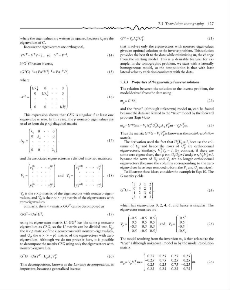
where the eigenvalues are written as squared because λ i are the
eigenvalues of G.
Because the eigenvectors are orthogonal,
VV T = V T V = I, so V T = V −1 .
(14)
If G
T G has an inverse,
(G T G) −1 = (VΛ 2 V T ) −1 = VΛ −2 V T ,
(15)
where
Λ
−
=
⋅ ⋅
⋅ ⋅
⋅
⋅
⋅ ⋅
⋅
⋅
⋅
⋅ ⋅
⋅
⋅ ⋅
⎛
⎝
⎜
⎜
⎜
⎜
⎜
⎞
⎠
⎟
⎟
⎟
⎟
⎟
2
1
2
2
2
2
1
0
0
0
1
0
0
0
1
/
/
/
.
λ
λ
λ r
(16)
This expression shows that G
T
G is singular if at least one
eigenvalue is zero. In this case, the p nonzero eigenvalues are
used to form the p × p diagonal matrix
Λ p
p
,
=
⋅ ⋅
⋅ ⋅
⋅
⋅ ⋅ ⋅ ⋅
⋅
⋅ ⋅ ⋅ ⋅
⋅ ⋅
⎛
⎝
⎜
⎜
⎜
⎜
⎜
⎞
⎠
⎟
⎟
⎟
⎟
⎟
λ
λ
λ
1
2
0
0
0
0
0 0
(17)
and the associated eigenvectors are divided into two matrices:
V
v
v
v
v
V
v
v
v
v
p
p
r
r
p
p
r
r
p
r
r
=
⋅ ⋅ ⋅
⋅ ⋅ ⋅ ⋅ ⋅
⋅ ⋅ ⋅ ⋅ ⋅
⋅ ⋅ ⋅ ⋅ ⋅
⋅ ⋅ ⋅
⎛
⎝
⎜
⎜
⎜
⎜
⎜
⎞
⎠
⎟
⎟
⎟
⎟
⎟
=
⋅ ⋅ ⋅
⋅
⋅ ⋅ ⋅ ⋅
⋅
⋅ ⋅ ⋅ ⋅
⋅
⋅ ⋅ ⋅ ⋅
⋅ ⋅ ⋅
⎛
⎝
⎜
⎜
⎜
⎜
⎜
⎞
+
+
( )
( )
( )
( )
( )
( )
( )
( )
1
1
1
1
0
1
1
1
1
and
⎠ ⎠
⎟
⎟
⎟
⎟
⎟
. (18)
V p is the r × p matrix of the eigenvectors with nonzero eigenvalues, and V 0 is the r × (r − p) matrix of the eigenvectors with
zero eigenvalues.
Similarly, the n × n matrix GG T can be decomposed as
GG
T = UΛ 2 U T ,
(19)
using its eigenvector matrix U. GG
T has the same p nonzero
eigenvalues as G T G, so the U matrix can be divided into U p ,
the n × p matrix of the eigenvectors with nonzero eigenvalues,
and U 0 , the n × (n − p) matrix of the eigenvectors with zero
eigenvalues. Although we do not prove it here, it is possible
to decompose the matrix G T G using only the eigenvectors with
nonzero eigenvalues:
G T G = UΛV T = U p Λ p V T
p .
(20)
This decomposition, known as the Lanczos decomposition, is
important, because a generalized inverse
G −p = V p Λ p
−1 U T
p
(21)
that involves only the eigenvectors with nonzero eigenvalues
gives an optimal solution to the inverse problem. This solution
provides the best fit to the data while minimizing m, the change
from the starting model. This is a desirable feature: for example, in the tomographic problem, we start with a laterally
homogeneous model, so the best solution is that with least
lateral velocity variation consistent with the data.
7.3.3 Properties of the generalized inverse solution
The relation between the solution to the inverse problem, the
model derived from the data using
m p = G −p d,
(22)
and the “true” (although unknown) model m, can be found
because the data are related to the “true” model by the forward
problem (Eqn 4), so
m p = G −p Gm = V p Λ p
−1 U T
p U p Λ p V T
p m = V p V T
p m.
(23)
Thus the matrix G −p G = V p V T
p is known as the model resolution
matrix.
The derivation used the fact that U T
p U p = I, because the columns of U p and hence the rows of U T
p are orthonormal
eigenvectors. Similarly, V
T
p V p = I. By contrast, if there are
some zero eigenvalues, then p ≠ n, U p U T
p ≠ I and p ≠ r, V p V T
p ≠ I,
because the rows of U p and V p are no longer orthonormal
eigenvectors (because the columns corresponding to the zero
eigenvalues have been removed to form the V 0 and U 0 matrices).
To illustrate these ideas, consider the example in Eqn 10. The
G matrix yields
G G
T
,
=
⎛
⎝
⎜
⎜
⎜
⎞
⎠
⎟
⎟
⎟
3 0 1 2
0 3 2 1
1 2 3 0
2 1 0 3
(24)
which has eigenvalues 0, 2, 4, 6, and hence is singular. The
eigenvector matrices are
V
V
p =
−
−
−
−
⎛
⎝
⎜
⎜
⎜
⎞
⎠
⎟
⎟
⎟
= −
−
⎛
⎝
⎜
⎜
⎜
⎞
⎠
⎟
⎟
⎟
.
.
.
.
.
.
.
.
.
.
.
.
.
.
.
.
.
0 5 0 5 0 5
0 5 0 5 0 5
0 5 0 5 0 5
0 5 0 5 0 5
0 5
0 5
0 5
0 5
0
and
(25)
The model resulting from the inversion m p is then related to the
“true” (although unknown) model m by the model resolution
matrix
m p = V p V T
p m =
0 75 0 25 0 25 0 25
0 25 0 75 0 25 0 25
0 25 0 25 0 75 0 25
0 25 0 25 0 25 0 75
.
.
.
.
.
.
.
.
.
.
.
.
.
.
.
.
.
−
−
−
−
⎛
⎝
⎜
⎜
⎜
⎞
⎠
⎟
⎟
⎟
m
(26)
7.3 Travel time tomography 427