

426 Inverse Problems
1
2
3
4
Block numbers
Seismometers
Ray path numbers
Seismometers
1
2
3
4
5
6
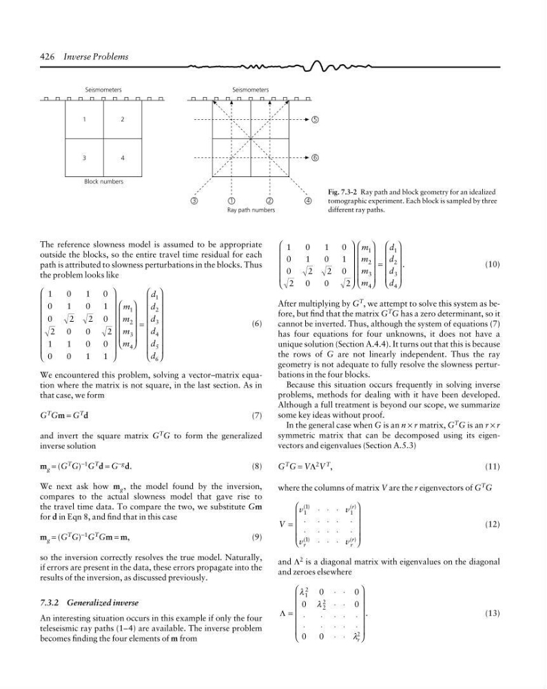
Fig. 7.3-2 Ray path and block geometry for an idealized
tomographic experiment. Each block is sampled by three
different ray paths.
The reference slowness model is assumed to be appropriate
outside the blocks, so the entire travel time residual for each
path is attributed to slowness perturbations in the blocks. Thus
the problem looks like
1
0
1
0
0
1
0
1
0
2
2 0
2 0
0
2
1
1
0
0
0
0
1
1
1
2
3
4
1
2
3
4
5
6
⎛
⎝
⎜
⎜
⎜
⎜
⎜
⎜
⎜
⎞
⎠
⎟
⎟
⎟
⎟
⎟
⎟
⎟
⎛
⎝
⎜
⎜
⎜
⎜
⎞
⎠
⎟
⎟
⎟
⎟
=
⎛
⎝
⎜
⎜
⎜
⎜
⎜
⎜
⎜
⎞
⎠
⎟
⎟
⎟
⎟
⎟
⎟
⎟
m
m
m
m
d
d
d
d
d
d
(6)
We encountered this problem, solving a vector–matrix equation where the matrix is not square, in the last section. As in
that case, we form
G T Gm = G T d
(7)
and invert the square matrix G T G to form the generalized
inverse solution
m g = (G T G) −1 G T d = G −g d.
(8)
We next ask how m g , the model found by the inversion,
compares to the actual slowness model that gave rise to
the travel time data. To compare the two, we substitute Gm
for d in Eqn 8, and find that in this case
m g = (G T G) −1 G T Gm = m,
(9)
so the inversion correctly resolves the true model. Naturally,
if errors are present in the data, these errors propagate into the
results of the inversion, as discussed previously.
7.3.2 Generalized inverse
An interesting situation occurs in this example if only the four
teleseismic ray paths (1–4) are available. The inverse problem
becomes finding the four elements of m from
1
0
1
0
0
1
0
1
0
2
2 0
2 0
0
2
1
2
3
4
1
2
3
4
.
⎛
⎝
⎜
⎜
⎜
⎜
⎞
⎠
⎟
⎟
⎟
⎟
⎛
⎝
⎜
⎜
⎜
⎜
⎞
⎠
⎟
⎟
⎟
⎟
=
⎛
⎝
⎜
⎜
⎜
⎜
⎞
⎠
⎟
⎟
⎟
⎟
m
m
m
m
d
d
d
d
(10)
After multiplying by G
T
, we attempt to solve this system as before, but find that the matrix G T G has a zero determinant, so it
cannot be inverted. Thus, although the system of equations (7)
has four equations for four unknowns, it does not have a
unique solution (Section A.4.4). It turns out that this is because
the rows of G are not linearly independent. Thus the ray
geometry is not adequate to fully resolve the slowness perturbations in the four blocks.
Because this situation occurs frequently in solving inverse
problems, methods for dealing with it have been developed.
Although a full treatment is beyond our scope, we summarize
some key ideas without proof.
In the general case when G is an n × r matrix, G T G is an r × r
symmetric matrix that can be decomposed using its eigenvectors and eigenvalues (Section A.5.3)
G T G = VΛ 2 V T ,
(11)
where the columns of matrix V are the r eigenvectors of G
T G
V
v
v
v
v
r
r
r
r
( )
( )
( )
( )
=
⋅ ⋅ ⋅
⋅ ⋅ ⋅ ⋅ ⋅
⋅ ⋅ ⋅ ⋅ ⋅
⋅ ⋅ ⋅
⎛
⎝
⎜
⎜
⎜
⎜
⎞
⎠
⎟
⎟
⎟
⎟
1
1
1
1
(12)
and Λ 2 is a diagonal matrix with eigenvalues on the diagonal
and zeroes elsewhere
Λ
.
=
⋅ ⋅
⋅ ⋅
⋅
⋅ ⋅ ⋅ ⋅
⋅
⋅ ⋅ ⋅ ⋅
⋅ ⋅
⎛
⎝
⎜
⎜
⎜
⎜
⎜
⎞
⎠
⎟
⎟
⎟
⎟
⎟
λ
λ
λ
1
2
2
2
2
0
0
0
0
0
0
r
(13)
1
2
3
4
Block numbers
Seismometers
Ray path numbers
Seismometers
1
2
3
4
5
6
Fig. 7.3-2 Ray path and block geometry for an idealized
tomographic experiment. Each block is sampled by three
different ray paths.
The reference slowness model is assumed to be appropriate
outside the blocks, so the entire travel time residual for each
path is attributed to slowness perturbations in the blocks. Thus
the problem looks like
1
0
1
0
0
1
0
1
0
2
2 0
2 0
0
2
1
1
0
0
0
0
1
1
1
2
3
4
1
2
3
4
5
6
⎛
⎝
⎜
⎜
⎜
⎜
⎜
⎜
⎜
⎞
⎠
⎟
⎟
⎟
⎟
⎟
⎟
⎟
⎛
⎝
⎜
⎜
⎜
⎜
⎞
⎠
⎟
⎟
⎟
⎟
=
⎛
⎝
⎜
⎜
⎜
⎜
⎜
⎜
⎜
⎞
⎠
⎟
⎟
⎟
⎟
⎟
⎟
⎟
m
m
m
m
d
d
d
d
d
d
(6)
We encountered this problem, solving a vector–matrix equation where the matrix is not square, in the last section. As in
that case, we form
G T Gm = G T d
(7)
and invert the square matrix G T G to form the generalized
inverse solution
m g = (G T G) −1 G T d = G −g d.
(8)
We next ask how m g , the model found by the inversion,
compares to the actual slowness model that gave rise to
the travel time data. To compare the two, we substitute Gm
for d in Eqn 8, and find that in this case
m g = (G T G) −1 G T Gm = m,
(9)
so the inversion correctly resolves the true model. Naturally,
if errors are present in the data, these errors propagate into the
results of the inversion, as discussed previously.
7.3.2 Generalized inverse
An interesting situation occurs in this example if only the four
teleseismic ray paths (1–4) are available. The inverse problem
becomes finding the four elements of m from
1
0
1
0
0
1
0
1
0
2
2 0
2 0
0
2
1
2
3
4
1
2
3
4
.
⎛
⎝
⎜
⎜
⎜
⎜
⎞
⎠
⎟
⎟
⎟
⎟
⎛
⎝
⎜
⎜
⎜
⎜
⎞
⎠
⎟
⎟
⎟
⎟
=
⎛
⎝
⎜
⎜
⎜
⎜
⎞
⎠
⎟
⎟
⎟
⎟
m
m
m
m
d
d
d
d
(10)
After multiplying by G
T
, we attempt to solve this system as before, but find that the matrix G T G has a zero determinant, so it
cannot be inverted. Thus, although the system of equations (7)
has four equations for four unknowns, it does not have a
unique solution (Section A.4.4). It turns out that this is because
the rows of G are not linearly independent. Thus the ray
geometry is not adequate to fully resolve the slowness perturbations in the four blocks.
Because this situation occurs frequently in solving inverse
problems, methods for dealing with it have been developed.
Although a full treatment is beyond our scope, we summarize
some key ideas without proof.
In the general case when G is an n × r matrix, G T G is an r × r
symmetric matrix that can be decomposed using its eigenvectors and eigenvalues (Section A.5.3)
G T G = VΛ 2 V T ,
(11)
where the columns of matrix V are the r eigenvectors of G
T G
V
v
v
v
v
r
r
r
r
( )
( )
( )
( )
=
⋅ ⋅ ⋅
⋅ ⋅ ⋅ ⋅ ⋅
⋅ ⋅ ⋅ ⋅ ⋅
⋅ ⋅ ⋅
⎛
⎝
⎜
⎜
⎜
⎜
⎞
⎠
⎟
⎟
⎟
⎟
1
1
1
1
(12)
and Λ 2 is a diagonal matrix with eigenvalues on the diagonal
and zeroes elsewhere
Λ
.
=
⋅ ⋅
⋅ ⋅
⋅
⋅ ⋅ ⋅ ⋅
⋅
⋅ ⋅ ⋅ ⋅
⋅ ⋅
⎛
⎝
⎜
⎜
⎜
⎜
⎜
⎞
⎠
⎟
⎟
⎟
⎟
⎟
λ
λ
λ
1
2
2
2
2
0
0
0
0
0
0
r
(13)