

is perturbed by an amount δu(s) small enough that the ray path
is essentially unchanged, but the travel time changes by
δT = Ύ δu(s)ds.
(2)
We can then use the changes in travel time to study the velocity
changes that caused them.
Because the travel time perturbation reflects the slowness
perturbation integrated along the ray path, a single observation
does not indicate how the perturbation is distributed along
the path. A large localized perturbation and a smaller, but more
widely distributed, one could give the same effect. To improve
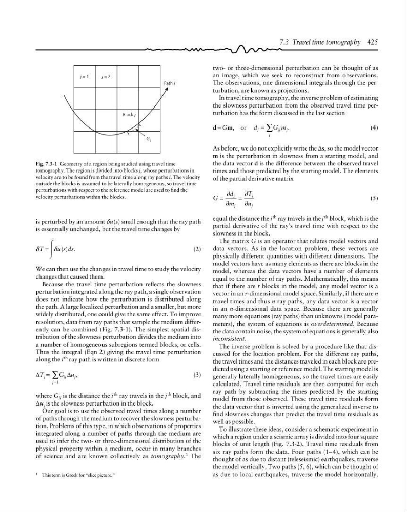
resolution, data from ray paths that sample the medium differently can be combined (Fig. 7.3-1). The simplest spatial distribution of the slowness perturbation divides the medium into
a number of homogeneous subregions termed blocks, or cells.
Thus the integral (Eqn 2) giving the travel time perturbation
along the i th ray path is written in discrete form
∆T i = G u
ij
j
j
∆ ,
=
∑
1
(3)
where G ij is the distance the i th ray travels in the j th block, and
∆u j is the slowness perturbation in the block.
Our goal is to use the observed travel times along a number
of paths through the medium to recover the slowness perturbation. Problems of this type, in which observations of properties
integrated along a number of paths through the medium are
used to infer the two- or three-dimensional distribution of the
physical property within a medium, occur in many branches
of science and are known collectively as tomography. 1 The
two- or three-dimensional perturbation can be thought of as
an image, which we seek to reconstruct from observations.
The observations, one-dimensional integrals through the perturbation, are known as projections.
In travel time tomography, the inverse problem of estimating
the slowness perturbation from the observed travel time perturbation has the form discussed in the last section
d = Gm, or d
G m
i
i j j
j
= ∑
.
(4)
As before, we do not explicitly write the ∆s, so the model vector
m is the perturbation in slowness from a starting model, and
the data vector d is the difference between the observed travel
times and those predicted by the starting model. The elements
of the partial derivative matrix
G
d
m
T
u
i
j
i
j
=
=
∂
∂
∂
∂
(5)
equal the distance the i
th ray travels in the j
th block, which is the
partial derivative of the ray’s travel time with respect to the
slowness in the block.
The matrix G is an operator that relates model vectors and
data vectors. As in the location problem, these vectors are
physically different quantities with different dimensions. The
model vectors have as many elements as there are blocks in the
model, whereas the data vectors have a number of elements
equal to the number of ray paths. Mathematically, this means
that if there are r blocks in the model, any model vector is a
vector in an r-dimensional model space. Similarly, if there are n
travel times and thus n ray paths, any data vector is a vector
in an n-dimensional data space. Because there are generally
many more equations (ray paths) than unknowns (model parameters), the system of equations is overdetermined. Because
the data contain noise, the system of equations is generally also
inconsistent.
The inverse problem is solved by a procedure like that discussed for the location problem. For the different ray paths,
the travel times and the distances traveled in each block are predicted using a starting or reference model. The starting model is
generally laterally homogeneous, so the travel times are easily
calculated. Travel time residuals are then computed for each
ray path by subtracting the times predicted by the starting
model from those observed. These travel time residuals form
the data vector that is inverted using the generalized inverse to
find slowness changes that predict the travel time residuals as
well as possible.
To illustrate these ideas, consider a schematic experiment in
which a region under a seismic array is divided into four square
blocks of unit length (Fig. 7.3-2). Travel time residuals from
six ray paths form the data. Four paths (1–4), which can be
thought of as due to distant (teleseismic) earthquakes, traverse
the model vertically. Two paths (5, 6), which can be thought of
as due to local earthquakes, traverse the model horizontally.
1 This term is Greek for “slice picture.”
Block j
j = 2
j = 1
Path i
G ij
Fig. 7.3-1 Geometry of a region being studied using travel time
tomography. The region is divided into blocks j, whose perturbations in
velocity are to be found from the travel time along ray paths i. The velocity
outside the blocks is assumed to be laterally homogeneous, so travel time
perturbations with respect to the reference model are used to find the
velocity perturbations within the blocks.
7.3 Travel time tomography 425
is essentially unchanged, but the travel time changes by
δT = Ύ δu(s)ds.
(2)
We can then use the changes in travel time to study the velocity
changes that caused them.
Because the travel time perturbation reflects the slowness
perturbation integrated along the ray path, a single observation
does not indicate how the perturbation is distributed along
the path. A large localized perturbation and a smaller, but more
widely distributed, one could give the same effect. To improve
resolution, data from ray paths that sample the medium differently can be combined (Fig. 7.3-1). The simplest spatial distribution of the slowness perturbation divides the medium into
a number of homogeneous subregions termed blocks, or cells.
Thus the integral (Eqn 2) giving the travel time perturbation
along the i th ray path is written in discrete form
∆T i = G u
ij
j
j
∆ ,
=
∑
1
(3)
where G ij is the distance the i th ray travels in the j th block, and
∆u j is the slowness perturbation in the block.
Our goal is to use the observed travel times along a number
of paths through the medium to recover the slowness perturbation. Problems of this type, in which observations of properties
integrated along a number of paths through the medium are
used to infer the two- or three-dimensional distribution of the
physical property within a medium, occur in many branches
of science and are known collectively as tomography. 1 The
two- or three-dimensional perturbation can be thought of as
an image, which we seek to reconstruct from observations.
The observations, one-dimensional integrals through the perturbation, are known as projections.
In travel time tomography, the inverse problem of estimating
the slowness perturbation from the observed travel time perturbation has the form discussed in the last section
d = Gm, or d
G m
i
i j j
j
= ∑
.
(4)
As before, we do not explicitly write the ∆s, so the model vector
m is the perturbation in slowness from a starting model, and
the data vector d is the difference between the observed travel
times and those predicted by the starting model. The elements
of the partial derivative matrix
G
d
m
T
u
i
j
i
j
=
=
∂
∂
∂
∂
(5)
equal the distance the i
th ray travels in the j
th block, which is the
partial derivative of the ray’s travel time with respect to the
slowness in the block.
The matrix G is an operator that relates model vectors and
data vectors. As in the location problem, these vectors are
physically different quantities with different dimensions. The
model vectors have as many elements as there are blocks in the
model, whereas the data vectors have a number of elements
equal to the number of ray paths. Mathematically, this means
that if there are r blocks in the model, any model vector is a
vector in an r-dimensional model space. Similarly, if there are n
travel times and thus n ray paths, any data vector is a vector
in an n-dimensional data space. Because there are generally
many more equations (ray paths) than unknowns (model parameters), the system of equations is overdetermined. Because
the data contain noise, the system of equations is generally also
inconsistent.
The inverse problem is solved by a procedure like that discussed for the location problem. For the different ray paths,
the travel times and the distances traveled in each block are predicted using a starting or reference model. The starting model is
generally laterally homogeneous, so the travel times are easily
calculated. Travel time residuals are then computed for each
ray path by subtracting the times predicted by the starting
model from those observed. These travel time residuals form
the data vector that is inverted using the generalized inverse to
find slowness changes that predict the travel time residuals as
well as possible.
To illustrate these ideas, consider a schematic experiment in
which a region under a seismic array is divided into four square
blocks of unit length (Fig. 7.3-2). Travel time residuals from
six ray paths form the data. Four paths (1–4), which can be
thought of as due to distant (teleseismic) earthquakes, traverse
the model vertically. Two paths (5, 6), which can be thought of
as due to local earthquakes, traverse the model horizontally.
1 This term is Greek for “slice picture.”
Block j
j = 2
j = 1
Path i
G ij
Fig. 7.3-1 Geometry of a region being studied using travel time
tomography. The region is divided into blocks j, whose perturbations in
velocity are to be found from the travel time along ray paths i. The velocity
outside the blocks is assumed to be laterally homogeneous, so travel time
perturbations with respect to the reference model are used to find the
velocity perturbations within the blocks.
7.3 Travel time tomography 425