

424 Inverse Problems
locate a group of nearby earthquakes using a travel time correction at each station derived from the residual at each station for
the master event. This procedure attempts to locate the other
events more accurately with respect to the master event. Joint
hypocenter determination methods use data from a number of
nearby earthquakes, and locate them simultaneously to best fit
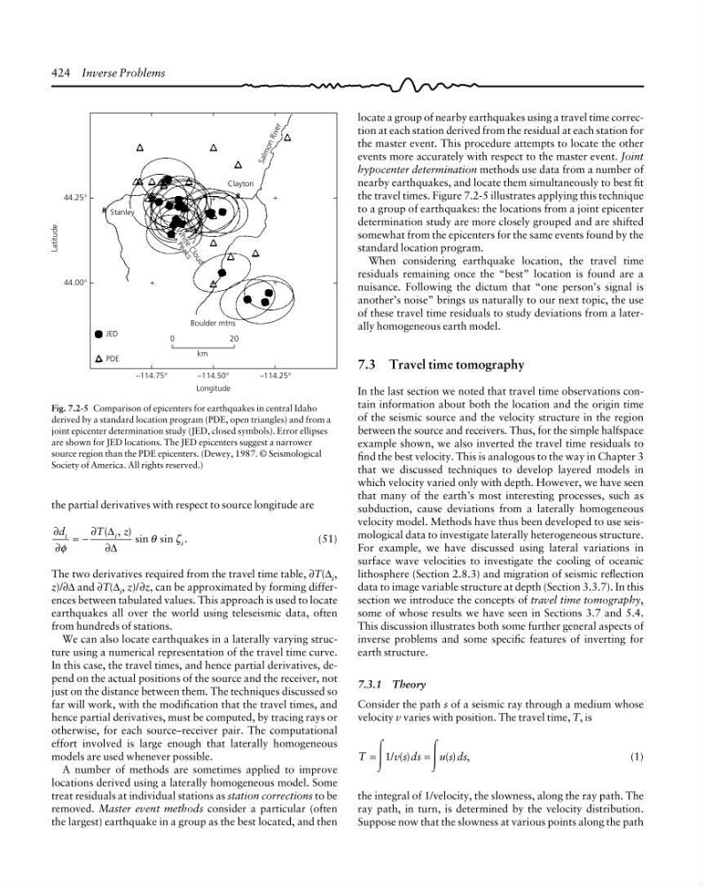
the travel times. Figure 7.2-5 illustrates applying this technique
to a group of earthquakes: the locations from a joint epicenter
determination study are more closely grouped and are shifted
somewhat from the epicenters for the same events found by the
standard location program.
When considering earthquake location, the travel time
residuals remaining once the “best” location is found are a
nuisance. Following the dictum that “one person’s signal is
another’s noise” brings us naturally to our next topic, the use
of these travel time residuals to study deviations from a laterally homogeneous earth model.
7.3 Travel time tomography
In the last section we noted that travel time observations contain information about both the location and the origin time
of the seismic source and the velocity structure in the region
between the source and receivers. Thus, for the simple halfspace
example shown, we also inverted the travel time residuals to
find the best velocity. This is analogous to the way in Chapter 3
that we discussed techniques to develop layered models in
which velocity varied only with depth. However, we have seen
that many of the earth’s most interesting processes, such as
subduction, cause deviations from a laterally homogeneous
velocity model. Methods have thus been developed to use seismological data to investigate laterally heterogeneous structure.
For example, we have discussed using lateral variations in
surface wave velocities to investigate the cooling of oceanic
lithosphere (Section 2.8.3) and migration of seismic reflection
data to image variable structure at depth (Section 3.3.7). In this
section we introduce the concepts of travel time tomography,
some of whose results we have seen in Sections 3.7 and 5.4.
This discussion illustrates both some further general aspects of
inverse problems and some specific features of inverting for
earth structure.
7.3.1 Theory
Consider the path s of a seismic ray through a medium whose
velocity v varies with position. The travel time, T, is
T
vsds
usds
/ ( )
( ) ,
=
=
Ύ
Ύ
1
(1)
the integral of 1/velocity, the slowness, along the ray path. The
ray path, in turn, is determined by the velocity distribution.
Suppose now that the slowness at various points along the path
–114.75°
Latitude
44.25°
# Stanley
Clayton
S a lm o n R iv e r
W
h
it
e
C
lo
u
d
P
e
a
k
s
Boulder mtns
0
2 0
km
–114.50°
–114.25°
Longitude
44.00°
+
+
#
+
+
+
JED
PDE
Fig. 7.2-5 Comparison of epicenters for earthquakes in central Idaho
derived by a standard location program (PDE, open triangles) and from a
joint epicenter determination study (JED, closed symbols). Error ellipses
are shown for JED locations. The JED epicenters suggest a narrower
source region than the PDE epicenters. (Dewey, 1987. © Seismological
Society of America. All rights reserved.)
the partial derivatives with respect to source longitude are
∂
∂
∂
∂
d
T
z
i
i
i
φ
θ
ζ
( , ) sin sin .
= −
∆
∆
(51)
The two derivatives required from the travel time table, ∂T(∆ i ,
z)/∂∆ and ∂T(∆ i , z)/∂z, can be approximated by forming differences between tabulated values. This approach is used to locate
earthquakes all over the world using teleseismic data, often
from hundreds of stations.
We can also locate earthquakes in a laterally varying structure using a numerical representation of the travel time curve.
In this case, the travel times, and hence partial derivatives, depend on the actual positions of the source and the receiver, not
just on the distance between them. The techniques discussed so
far will work, with the modification that the travel times, and
hence partial derivatives, must be computed, by tracing rays or
otherwise, for each source–receiver pair. The computational
effort involved is large enough that laterally homogeneous
models are used whenever possible.
A number of methods are sometimes applied to improve
locations derived using a laterally homogeneous model. Some
treat residuals at individual stations as station corrections to be
removed. Master event methods consider a particular (often
the largest) earthquake in a group as the best located, and then
locate a group of nearby earthquakes using a travel time correction at each station derived from the residual at each station for
the master event. This procedure attempts to locate the other
events more accurately with respect to the master event. Joint
hypocenter determination methods use data from a number of
nearby earthquakes, and locate them simultaneously to best fit
the travel times. Figure 7.2-5 illustrates applying this technique
to a group of earthquakes: the locations from a joint epicenter
determination study are more closely grouped and are shifted
somewhat from the epicenters for the same events found by the
standard location program.
When considering earthquake location, the travel time
residuals remaining once the “best” location is found are a
nuisance. Following the dictum that “one person’s signal is
another’s noise” brings us naturally to our next topic, the use
of these travel time residuals to study deviations from a laterally homogeneous earth model.
7.3 Travel time tomography
In the last section we noted that travel time observations contain information about both the location and the origin time
of the seismic source and the velocity structure in the region
between the source and receivers. Thus, for the simple halfspace
example shown, we also inverted the travel time residuals to
find the best velocity. This is analogous to the way in Chapter 3
that we discussed techniques to develop layered models in
which velocity varied only with depth. However, we have seen
that many of the earth’s most interesting processes, such as
subduction, cause deviations from a laterally homogeneous
velocity model. Methods have thus been developed to use seismological data to investigate laterally heterogeneous structure.
For example, we have discussed using lateral variations in
surface wave velocities to investigate the cooling of oceanic
lithosphere (Section 2.8.3) and migration of seismic reflection
data to image variable structure at depth (Section 3.3.7). In this
section we introduce the concepts of travel time tomography,
some of whose results we have seen in Sections 3.7 and 5.4.
This discussion illustrates both some further general aspects of
inverse problems and some specific features of inverting for
earth structure.
7.3.1 Theory
Consider the path s of a seismic ray through a medium whose
velocity v varies with position. The travel time, T, is
T
vsds
usds
/ ( )
( ) ,
=
=
Ύ
Ύ
1
(1)
the integral of 1/velocity, the slowness, along the ray path. The
ray path, in turn, is determined by the velocity distribution.
Suppose now that the slowness at various points along the path
–114.75°
Latitude
44.25°
# Stanley
Clayton
S a lm o n R iv e r
W
h
it
e
C
lo
u
d
P
e
a
k
s
Boulder mtns
0
2 0
km
–114.50°
–114.25°
Longitude
44.00°
+
+
#
+
+
+
JED
PDE
Fig. 7.2-5 Comparison of epicenters for earthquakes in central Idaho
derived by a standard location program (PDE, open triangles) and from a
joint epicenter determination study (JED, closed symbols). Error ellipses
are shown for JED locations. The JED epicenters suggest a narrower
source region than the PDE epicenters. (Dewey, 1987. © Seismological
Society of America. All rights reserved.)
the partial derivatives with respect to source longitude are
∂
∂
∂
∂
d
T
z
i
i
i
φ
θ
ζ
( , ) sin sin .
= −
∆
∆
(51)
The two derivatives required from the travel time table, ∂T(∆ i ,
z)/∂∆ and ∂T(∆ i , z)/∂z, can be approximated by forming differences between tabulated values. This approach is used to locate
earthquakes all over the world using teleseismic data, often
from hundreds of stations.
We can also locate earthquakes in a laterally varying structure using a numerical representation of the travel time curve.
In this case, the travel times, and hence partial derivatives, depend on the actual positions of the source and the receiver, not
just on the distance between them. The techniques discussed so
far will work, with the modification that the travel times, and
hence partial derivatives, must be computed, by tracing rays or
otherwise, for each source–receiver pair. The computational
effort involved is large enough that laterally homogeneous
models are used whenever possible.
A number of methods are sometimes applied to improve
locations derived using a laterally homogeneous model. Some
treat residuals at individual stations as station corrections to be
removed. Master event methods consider a particular (often
the largest) earthquake in a group as the best located, and then