

The location of earthquakes for a spherical earth is similar.
As before, we assume that velocity varies only with depth. In
this case, for an earthquake at colatitude θ, longitude φ, focal
depth z, and origin time t, we seek to estimate the model vector
m = (θ, φ, z, t) from the data.
The travel time to receivers on the surface at colatitudes θ i
and longitude φ i depends on the focal depth and the angular
distance from the epicenter (Eqn A.7.7),
cos ∆ i = cos θ cos θ i + sin θ sin θ i cos (φ i − φ).
(44)
For a travel time curve T(∆, z) the arrival times are
d i = T(∆ i , z) + t.
(45)
Several average global travel time curves are available, as in
Fig. 3.5-4. In addition, a travel time curve for a specific velocity
model can be found numerically by tracing rays.
In this case, the θ derivatives are found using
∂
∂
∂
∂
∂
∂
∂
∂
d
T
z
T
z
i
i
i
i
i
θ
θ
θ
( , )
( , )
.
=
=
∆
∆
∆
∆
∆
(46)
To find the last term, note that
∂
∂
∂
∂
∂
∂
(cos )
(cos ) ( ) ,
∆
∆
∆
∆
i
i
i
θ
θ
=
(47)
so
∂
∂
∂
∂
∂
∂
( )
(cos )
(cos )
∆
∆
∆
∆
i
i
i
θ
θ
=
⎛
⎝
⎜
⎞
⎠
⎟
⎛
⎝
⎜
⎞
⎠
⎟
=
sin
1
∆ i
(sin θ cos θ i − cos θ sin θ i cos (φ i − φ))
= cos ζ i ,
(48)
where ζ i is the azimuth of the i th station with respect to the
earthquake (Eqn. A.7.10). Thus the partial derivatives with
respect to source colatitude are
∂
∂
∂
∂
d
T
z
i
i
i
θ
ζ
( , ) cos .
=
∆
∆
(49)
Similarly, because by the same method
∂
∂
∂
∂
∂
∂
( )
(cos )
(cos )
∆
∆
∆
∆
i
i
i
φ
φ
=
⎛
⎝
⎜
⎞
⎠
⎟
⎛
⎝
⎜
⎞
⎠
⎟
=
sin
1
∆ i
(−sin θ sin θ i sin (φ i − φ))
= −sin θ sin ζ i ,
(50)
Earthquake
epicenter
(x, y)
r
ξ
y
x
Station
(x i , y i )
Fig. 7.2-4 Map view of the relation between an earthquake epicenter and
a seismic station in Cartesian coordinates.
and the source depth z, so the arrival times are
d i ′ = T(r i , z) + t.
(39)
In this case, the x derivatives are found by
∂
∂
∂
∂
∂
∂
∂
∂
∂
∂
d
x
T r z
x
T r z
r
r
x
T r z
r
x x
r
i
i
i
i
i
i
i
( , )
( , )
( , ) (
) ,
=
=
=
−
(40)
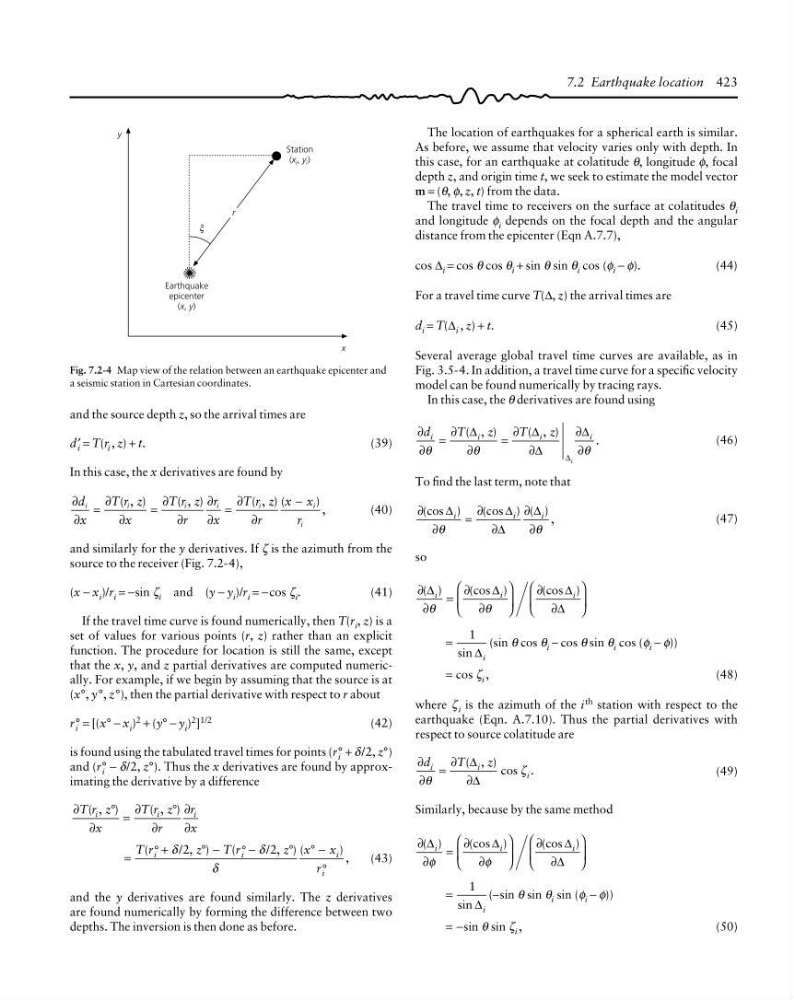
and similarly for the y derivatives. If ζ is the azimuth from the
source to the receiver (Fig. 7.2-4),
(x − x i )/r i = −sin ζ i and (y − y i )/r i = −cos ζ i .
(41)
If the travel time curve is found numerically, then T(r i , z) is a
set of values for various points (r, z) rather than an explicit
function. The procedure for location is still the same, except
that the x, y, and z partial derivatives are computed numerically. For example, if we begin by assuming that the source is at
(x°, y°, z°), then the partial derivative with respect to r about
r i
° = [(x° − x i ) 2 + (y° − y i ) 2 ] 1/2
(42)
is found using the tabulated travel times for points (r i
° + δ /2, z°)
and (r i
° − δ/2, z°). Thus the x derivatives are found by approximating the derivative by a difference
∂
∂
∂
∂
∂
∂
T r z
x
T r z
r
r
x
i
i
i
( , )
( , )
°
°
=
=
+
−
−
−
(
/ , )
(
/ , ) (
) ,
T r
z
T r
z x
x
r
i
i
i
i
°
°
°
° °
°
δ
δ
δ
2
2
(43)
and the y derivatives are found similarly. The z derivatives
are found numerically by forming the difference between two
depths. The inversion is then done as before.
7.2 Earthquake location 423
As before, we assume that velocity varies only with depth. In
this case, for an earthquake at colatitude θ, longitude φ, focal
depth z, and origin time t, we seek to estimate the model vector
m = (θ, φ, z, t) from the data.
The travel time to receivers on the surface at colatitudes θ i
and longitude φ i depends on the focal depth and the angular
distance from the epicenter (Eqn A.7.7),
cos ∆ i = cos θ cos θ i + sin θ sin θ i cos (φ i − φ).
(44)
For a travel time curve T(∆, z) the arrival times are
d i = T(∆ i , z) + t.
(45)
Several average global travel time curves are available, as in
Fig. 3.5-4. In addition, a travel time curve for a specific velocity
model can be found numerically by tracing rays.
In this case, the θ derivatives are found using
∂
∂
∂
∂
∂
∂
∂
∂
d
T
z
T
z
i
i
i
i
i
θ
θ
θ
( , )
( , )
.
=
=
∆
∆
∆
∆
∆
(46)
To find the last term, note that
∂
∂
∂
∂
∂
∂
(cos )
(cos ) ( ) ,
∆
∆
∆
∆
i
i
i
θ
θ
=
(47)
so
∂
∂
∂
∂
∂
∂
( )
(cos )
(cos )
∆
∆
∆
∆
i
i
i
θ
θ
=
⎛
⎝
⎜
⎞
⎠
⎟
⎛
⎝
⎜
⎞
⎠
⎟
=
sin
1
∆ i
(sin θ cos θ i − cos θ sin θ i cos (φ i − φ))
= cos ζ i ,
(48)
where ζ i is the azimuth of the i th station with respect to the
earthquake (Eqn. A.7.10). Thus the partial derivatives with
respect to source colatitude are
∂
∂
∂
∂
d
T
z
i
i
i
θ
ζ
( , ) cos .
=
∆
∆
(49)
Similarly, because by the same method
∂
∂
∂
∂
∂
∂
( )
(cos )
(cos )
∆
∆
∆
∆
i
i
i
φ
φ
=
⎛
⎝
⎜
⎞
⎠
⎟
⎛
⎝
⎜
⎞
⎠
⎟
=
sin
1
∆ i
(−sin θ sin θ i sin (φ i − φ))
= −sin θ sin ζ i ,
(50)
Earthquake
epicenter
(x, y)
r
ξ
y
x
Station
(x i , y i )
Fig. 7.2-4 Map view of the relation between an earthquake epicenter and
a seismic station in Cartesian coordinates.
and the source depth z, so the arrival times are
d i ′ = T(r i , z) + t.
(39)
In this case, the x derivatives are found by
∂
∂
∂
∂
∂
∂
∂
∂
∂
∂
d
x
T r z
x
T r z
r
r
x
T r z
r
x x
r
i
i
i
i
i
i
i
( , )
( , )
( , ) (
) ,
=
=
=
−
(40)
and similarly for the y derivatives. If ζ is the azimuth from the
source to the receiver (Fig. 7.2-4),
(x − x i )/r i = −sin ζ i and (y − y i )/r i = −cos ζ i .
(41)
If the travel time curve is found numerically, then T(r i , z) is a
set of values for various points (r, z) rather than an explicit
function. The procedure for location is still the same, except
that the x, y, and z partial derivatives are computed numerically. For example, if we begin by assuming that the source is at
(x°, y°, z°), then the partial derivative with respect to r about
r i
° = [(x° − x i ) 2 + (y° − y i ) 2 ] 1/2
(42)
is found using the tabulated travel times for points (r i
° + δ /2, z°)
and (r i
° − δ/2, z°). Thus the x derivatives are found by approximating the derivative by a difference
∂
∂
∂
∂
∂
∂
T r z
x
T r z
r
r
x
i
i
i
( , )
( , )
°
°
=
=
+
−
−
−
(
/ , )
(
/ , ) (
) ,
T r
z
T r
z x
x
r
i
i
i
i
°
°
°
° °
°
δ
δ
δ
2
2
(43)
and the y derivatives are found similarly. The z derivatives
are found numerically by forming the difference between two
depths. The inversion is then done as before.
7.2 Earthquake location 423