

420 Inverse Problems
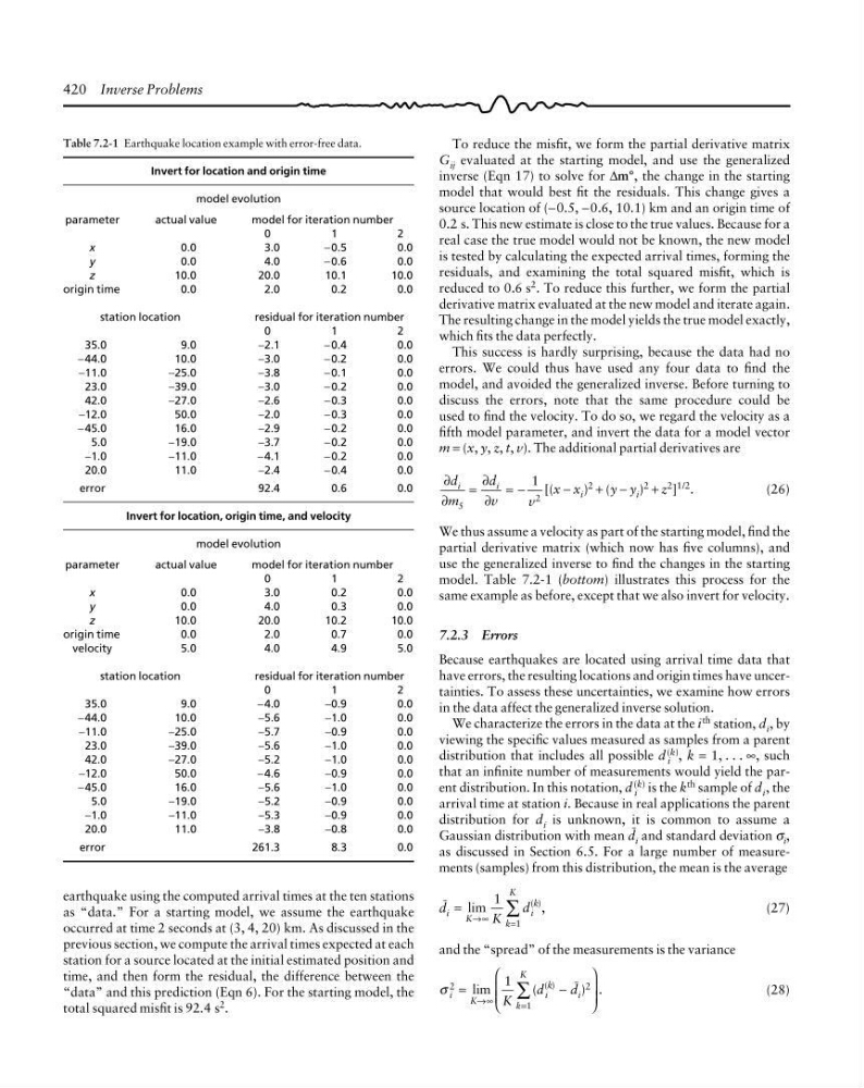
To reduce the misfit, we form the partial derivative matrix
G ij evaluated at the starting model, and use the generalized
inverse (Eqn 17) to solve for ∆m°, the change in the starting
model that would best fit the residuals. This change gives a
source location of (−0.5, −0.6, 10.1) km and an origin time of
0.2 s. This new estimate is close to the true values. Because for a
real case the true model would not be known, the new model
is tested by calculating the expected arrival times, forming the
residuals, and examining the total squared misfit, which is
reduced to 0.6 s 2 . To reduce this further, we form the partial
derivative matrix evaluated at the new model and iterate again.
The resulting change in the model yields the true model exactly,
which fits the data perfectly.
This success is hardly surprising, because the data had no
errors. We could thus have used any four data to find the
model, and avoided the generalized inverse. Before turning to
discuss the errors, note that the same procedure could be
used to find the velocity. To do so, we regard the velocity as a
fifth model parameter, and invert the data for a model vector
m = (x, y, z, t, v). The additional partial derivatives are
∂
∂
∂
∂
d
m
d
v
v
i
i
5
2
1
=
= − [(x − x i )
2
+ (y − y i )
2
+ z
2
]
1/2
.
(26)
We thus assume a velocity as part of the starting model, find the
partial derivative matrix (which now has five columns), and
use the generalized inverse to find the changes in the starting
model. Table 7.2-1 (bottom) illustrates this process for the
same example as before, except that we also invert for velocity.
7.2.3 Errors
Because earthquakes are located using arrival time data that
have errors, the resulting locations and origin times have uncertainties. To assess these uncertainties, we examine how errors
in the data affect the generalized inverse solution.
We characterize the errors in the data at the i th station, d i , by
viewing the specific values measured as samples from a parent
distribution that includes all possible d i
(k) , k = 1, . . . ∞, such
that an infinite number of measurements would yield the parent distribution. In this notation, d i
(k) is the k
th sample of d i , the
arrival time at station i. Because in real applications the parent
distribution for d i is unknown, it is common to assume a
Gaussian distribution with mean R i and standard deviation σ i ,
as discussed in Section 6.5. For a large number of measurements (samples) from this distribution, the mean is the average
R i =
→∞
=
∑
lim
,
( )
K
i
k
k
K
K
d
1
1
(27)
and the “spread” of the measurements is the variance
σ i K
i
k
i
k
K
K
d
2
2
1
1
=
−
⎛
⎝
⎜
⎜
⎞
⎠
⎟
⎟
→∞
=
∑
lim
(
) .
( )
R
(28)
Table 7.2-1 Earthquake location example with error-free data.
Invert for location and origin time
model evolution
parameter
actual value
model for iteration number
0
1
2
x
0.0
3.0
−0.5
0.0
y
0.0
4.0
−0.6
0.0
z
10.0
20.0
10.1
10.0
origin time
0.0
2.0
0.2
0.0
station location
residual for iteration number
0
1
2
35.0
9.0
−2.1
−0.4
0.0
−44.0
10.0
−3.0
−0.2
0.0
−11.0
−25.0
−3.8
−0.1
0.0
23.0
−39.0
−3.0
−0.2
0.0
42.0
−27.0
−2.6
−0.3
0.0
−12.0
50.0
−2.0
−0.3
0.0
−45.0
16.0
−2.9
−0.2
0.0
5.0
−19.0
−3.7
−0.2
0.0
−1.0
−11.0
−4.1
−0.2
0.0
20.0
11.0
−2.4
−0.4
0.0
error
92.4
0.6
0.0
Invert for location, origin time, and velocity
model evolution
parameter
actual value
model for iteration number
0
1
2
x
0.0
3.0
0.2
0.0
y
0.0
4.0
0.3
0.0
z
10.0
20.0
10.2
10.0
origin time
0.0
2.0
0.7
0.0
velocity
5.0
4.0
4.9
5.0
station location
residual for iteration number
0
1
2
35.0
9.0
−4.0
−0.9
0.0
−44.0
10.0
−5.6
−1.0
0.0
−11.0
−25.0
−5.7
−0.9
0.0
23.0
−39.0
−5.6
−1.0
0.0
42.0
−27.0
−5.2
−1.0
0.0
−12.0
50.0
−4.6
−0.9
0.0
−45.0
16.0
−5.6
−1.0
0.0
5.0
−19.0
−5.2
−0.9
0.0
−1.0
−11.0
−5.3
−0.9
0.0
20.0
11.0
−3.8
−0.8
0.0
error
261.3
8.3
0.0
earthquake using the computed arrival times at the ten stations
as “data.” For a starting model, we assume the earthquake
occurred at time 2 seconds at (3, 4, 20) km. As discussed in the
previous section, we compute the arrival times expected at each
station for a source located at the initial estimated position and
time, and then form the residual, the difference between the
“data” and this prediction (Eqn 6). For the starting model, the
total squared misfit is 92.4 s 2 .
To reduce the misfit, we form the partial derivative matrix
G ij evaluated at the starting model, and use the generalized
inverse (Eqn 17) to solve for ∆m°, the change in the starting
model that would best fit the residuals. This change gives a
source location of (−0.5, −0.6, 10.1) km and an origin time of
0.2 s. This new estimate is close to the true values. Because for a
real case the true model would not be known, the new model
is tested by calculating the expected arrival times, forming the
residuals, and examining the total squared misfit, which is
reduced to 0.6 s 2 . To reduce this further, we form the partial
derivative matrix evaluated at the new model and iterate again.
The resulting change in the model yields the true model exactly,
which fits the data perfectly.
This success is hardly surprising, because the data had no
errors. We could thus have used any four data to find the
model, and avoided the generalized inverse. Before turning to
discuss the errors, note that the same procedure could be
used to find the velocity. To do so, we regard the velocity as a
fifth model parameter, and invert the data for a model vector
m = (x, y, z, t, v). The additional partial derivatives are
∂
∂
∂
∂
d
m
d
v
v
i
i
5
2
1
=
= − [(x − x i )
2
+ (y − y i )
2
+ z
2
]
1/2
.
(26)
We thus assume a velocity as part of the starting model, find the
partial derivative matrix (which now has five columns), and
use the generalized inverse to find the changes in the starting
model. Table 7.2-1 (bottom) illustrates this process for the
same example as before, except that we also invert for velocity.
7.2.3 Errors
Because earthquakes are located using arrival time data that
have errors, the resulting locations and origin times have uncertainties. To assess these uncertainties, we examine how errors
in the data affect the generalized inverse solution.
We characterize the errors in the data at the i th station, d i , by
viewing the specific values measured as samples from a parent
distribution that includes all possible d i
(k) , k = 1, . . . ∞, such
that an infinite number of measurements would yield the parent distribution. In this notation, d i
(k) is the k
th sample of d i , the
arrival time at station i. Because in real applications the parent
distribution for d i is unknown, it is common to assume a
Gaussian distribution with mean R i and standard deviation σ i ,
as discussed in Section 6.5. For a large number of measurements (samples) from this distribution, the mean is the average
R i =
→∞
=
∑
lim
,
( )
K
i
k
k
K
K
d
1
1
(27)
and the “spread” of the measurements is the variance
σ i K
i
k
i
k
K
K
d
2
2
1
1
=
−
⎛
⎝
⎜
⎜
⎞
⎠
⎟
⎟
→∞
=
∑
lim
(
) .
( )
R
(28)
Table 7.2-1 Earthquake location example with error-free data.
Invert for location and origin time
model evolution
parameter
actual value
model for iteration number
0
1
2
x
0.0
3.0
−0.5
0.0
y
0.0
4.0
−0.6
0.0
z
10.0
20.0
10.1
10.0
origin time
0.0
2.0
0.2
0.0
station location
residual for iteration number
0
1
2
35.0
9.0
−2.1
−0.4
0.0
−44.0
10.0
−3.0
−0.2
0.0
−11.0
−25.0
−3.8
−0.1
0.0
23.0
−39.0
−3.0
−0.2
0.0
42.0
−27.0
−2.6
−0.3
0.0
−12.0
50.0
−2.0
−0.3
0.0
−45.0
16.0
−2.9
−0.2
0.0
5.0
−19.0
−3.7
−0.2
0.0
−1.0
−11.0
−4.1
−0.2
0.0
20.0
11.0
−2.4
−0.4
0.0
error
92.4
0.6
0.0
Invert for location, origin time, and velocity
model evolution
parameter
actual value
model for iteration number
0
1
2
x
0.0
3.0
0.2
0.0
y
0.0
4.0
0.3
0.0
z
10.0
20.0
10.2
10.0
origin time
0.0
2.0
0.7
0.0
velocity
5.0
4.0
4.9
5.0
station location
residual for iteration number
0
1
2
35.0
9.0
−4.0
−0.9
0.0
−44.0
10.0
−5.6
−1.0
0.0
−11.0
−25.0
−5.7
−0.9
0.0
23.0
−39.0
−5.6
−1.0
0.0
42.0
−27.0
−5.2
−1.0
0.0
−12.0
50.0
−4.6
−0.9
0.0
−45.0
16.0
−5.6
−1.0
0.0
5.0
−19.0
−5.2
−0.9
0.0
−1.0
−11.0
−5.3
−0.9
0.0
20.0
11.0
−3.8
−0.8
0.0
error
261.3
8.3
0.0
earthquake using the computed arrival times at the ten stations
as “data.” For a starting model, we assume the earthquake
occurred at time 2 seconds at (3, 4, 20) km. As discussed in the
previous section, we compute the arrival times expected at each
station for a source located at the initial estimated position and
time, and then form the residual, the difference between the
“data” and this prediction (Eqn 6). For the starting model, the
total squared misfit is 92.4 s 2 .