

If the Gaussian parent distribution is an appropriate choice,
there is a 68% probability that any sample will fall in the range
R i ± σ i , and a 95% probability that any sample will fall in the
range R i ± 2σ i (Fig. 6.5-1).
The errors at different stations are described by the variance–
covariance matrix of the data
σ
2
d = σ
2
d ij
= lim
K
k
K
K
→∞
=
∑
1
1
(d i
(k)
− R i )(d j
(k)
− R j ).
(29)
The diagonal (i = j) terms are the variances for data at
individual stations. The off-diagonal terms (i ≠ j) are the
covariances that describe the relation between errors at pairs
of stations. If the errors are uncorrelated between two stations
a for example, those due to a station clock a then how a
measurement at one station differs from the mean there is
unrelated to what occurs at another station, so their covariance
is ideally zero. Given a finite number of real data, we expect the
covariance to be small. By contrast, if the errors are correlated
(for example, if one person were reading seismograms from
different stations with a consistent bias), then similar deviations from the mean occur between these stations, and their
covariances would be larger. Errors can also be anti-correlated,
such that deviations at a station tend to occur in one direction,
whereas those at another station tend the other way, yielding
negative covariances. Although errors of measurement are likely
to be uncorrelated, systematic errors are often correlated. For
example, variations in velocity can cause systematic biases that
are either correlated or anti-correlated between different stations.
The data are inverted using the generalized inverse solution
m j =
G d
ji
g
i
i
−
∑
(30)
(here the ∆s are not written). As a result, the uncertainty in
a model parameter can reflect errors in all of the data. Thus,
even if the errors in the data are uncorrelated, the resulting
uncertainties in model parameters can be correlated. To see
this, we write the covariances of the model parameters in terms
of those for the data
σ 2
m = σ 2
mji = lim
K
k
K
K
→∞
=
∑
1
1
(m j
(k) − H j )(m i
(k) − H i )
=
−
⎛
⎝
⎜ ⎜
⎞
⎠
⎟ ⎟
−
⎛
⎝
⎜
⎞
⎠
⎟
→∞
−
=
−
∑
∑
∑
lim
(
)
(
)
( )
( )
K
jp
g
p
k
p
p
k
K
is
g
s
k
s
s
K
G d
G d
1
1
R
R
=
−
−
⎛
⎝
⎜
⎜
⎞
⎠
⎟
⎟
−
−
→∞
=
∑ ∑
∑
lim
(
)(
)
( )
( )
G
G
K
d
d
jp
g
p
is
g
s
K
p
k
p
s
k
s
k
K
1
1
R
R
=
−
−
∑ ∑
.
G
G
jp
g
p
is
g
d
s
ps
σ 2
(31)
This relation can be written in matrix form in terms of σ d
2 and
σ m
2 , the variance–covariance matrices for the data and model:
σ 2
m = G −g σ d
2 (G −g ) T .
(32)
We often assume that the data errors are uncorrelated and
equal, so that the data variance–covariance matrix is a constant times the identity matrix,
σ d
2 = σ 2 δ ij ,
(33)
and the model variance–covariance matrix is
σ m
2 = σ 2 (G T G) −1 ,
(34)
as proved in problem 4.
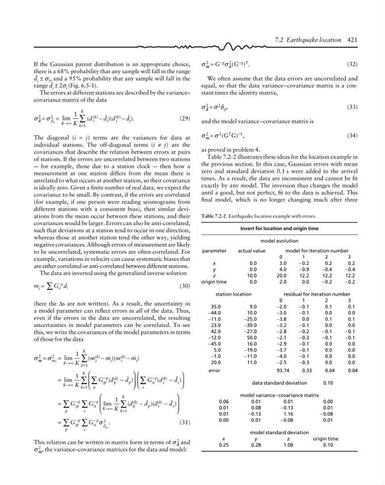
Table 7.2-2 illustrates these ideas for the location example in
the previous section. In this case, Gaussian errors with mean
zero and standard deviation 0.1 s were added to the arrival
times. As a result, the data are inconsistent and cannot be fit
exactly by any model. The inversion thus changes the model
until a good, but not perfect, fit to the data is achieved. This
final model, which is no longer changing much after three
Table 7.2-2 Earthquake location example with errors.
Invert for location and origin time
model evolution
parameter
actual value
model for iteration number
0
1
2
3
x
0.0
3.0
−0.2
0.2
0.2
y
0.0
4.0
−0.9
−0.4
−0.4
z
10.0
20.0
12.2
12.2
12.2
origin time
0.0
2.0
0.0
−0.2
−0.2
station location
residual for iteration number
0
1
2
3
35.0
9.0
−2.0
−0.1
0.1
0.1
−44.0
10.0
−3.0
−0.1
0.0
0.0
−11.0
−25.0
−3.8
0.0
0.1
0.1
23.0
−39.0
−3.2
−0.1
0.0
0.0
42.0
−27.0
−2.8
−0.2
−0.1
−0.1
−12.0
50.0
−2.1
−0.3
−0.1
−0.1
−45.0
16.0
−2.9
−0.1
0.0
0.0
5.0
−19.0
−3.7
−0.1
0.0
0.0
−1.0
−11.0
−4.0
−0.1
0.0
0.0
20.0
11.0
−2.5
−0.3
0.0
0.0
error
93.74
0.33
0.04
0.04
data standard deviation
0.10
model variance–covariance matrix
0.06
0.01
0.01
0.00
0.01
0.08
−0.13
0.01
0.01
−0.13
1.16
−0.08
0.00
0.01
−0.08
0.01
model standard deviation
x
y
z
origin time
0.25
0.28
1.08
0.10
7.2 Earthquake location 421
there is a 68% probability that any sample will fall in the range
R i ± σ i , and a 95% probability that any sample will fall in the
range R i ± 2σ i (Fig. 6.5-1).
The errors at different stations are described by the variance–
covariance matrix of the data
σ
2
d = σ
2
d ij
= lim
K
k
K
K
→∞
=
∑
1
1
(d i
(k)
− R i )(d j
(k)
− R j ).
(29)
The diagonal (i = j) terms are the variances for data at
individual stations. The off-diagonal terms (i ≠ j) are the
covariances that describe the relation between errors at pairs
of stations. If the errors are uncorrelated between two stations
a for example, those due to a station clock a then how a
measurement at one station differs from the mean there is
unrelated to what occurs at another station, so their covariance
is ideally zero. Given a finite number of real data, we expect the
covariance to be small. By contrast, if the errors are correlated
(for example, if one person were reading seismograms from
different stations with a consistent bias), then similar deviations from the mean occur between these stations, and their
covariances would be larger. Errors can also be anti-correlated,
such that deviations at a station tend to occur in one direction,
whereas those at another station tend the other way, yielding
negative covariances. Although errors of measurement are likely
to be uncorrelated, systematic errors are often correlated. For
example, variations in velocity can cause systematic biases that
are either correlated or anti-correlated between different stations.
The data are inverted using the generalized inverse solution
m j =
G d
ji
g
i
i
−
∑
(30)
(here the ∆s are not written). As a result, the uncertainty in
a model parameter can reflect errors in all of the data. Thus,
even if the errors in the data are uncorrelated, the resulting
uncertainties in model parameters can be correlated. To see
this, we write the covariances of the model parameters in terms
of those for the data
σ 2
m = σ 2
mji = lim
K
k
K
K
→∞
=
∑
1
1
(m j
(k) − H j )(m i
(k) − H i )
=
−
⎛
⎝
⎜ ⎜
⎞
⎠
⎟ ⎟
−
⎛
⎝
⎜
⎞
⎠
⎟
→∞
−
=
−
∑
∑
∑
lim
(
)
(
)
( )
( )
K
jp
g
p
k
p
p
k
K
is
g
s
k
s
s
K
G d
G d
1
1
R
R
=
−
−
⎛
⎝
⎜
⎜
⎞
⎠
⎟
⎟
−
−
→∞
=
∑ ∑
∑
lim
(
)(
)
( )
( )
G
G
K
d
d
jp
g
p
is
g
s
K
p
k
p
s
k
s
k
K
1
1
R
R
=
−
−
∑ ∑
.
G
G
jp
g
p
is
g
d
s
ps
σ 2
(31)
This relation can be written in matrix form in terms of σ d
2 and
σ m
2 , the variance–covariance matrices for the data and model:
σ 2
m = G −g σ d
2 (G −g ) T .
(32)
We often assume that the data errors are uncorrelated and
equal, so that the data variance–covariance matrix is a constant times the identity matrix,
σ d
2 = σ 2 δ ij ,
(33)
and the model variance–covariance matrix is
σ m
2 = σ 2 (G T G) −1 ,
(34)
as proved in problem 4.
Table 7.2-2 illustrates these ideas for the location example in
the previous section. In this case, Gaussian errors with mean
zero and standard deviation 0.1 s were added to the arrival
times. As a result, the data are inconsistent and cannot be fit
exactly by any model. The inversion thus changes the model
until a good, but not perfect, fit to the data is achieved. This
final model, which is no longer changing much after three
Table 7.2-2 Earthquake location example with errors.
Invert for location and origin time
model evolution
parameter
actual value
model for iteration number
0
1
2
3
x
0.0
3.0
−0.2
0.2
0.2
y
0.0
4.0
−0.9
−0.4
−0.4
z
10.0
20.0
12.2
12.2
12.2
origin time
0.0
2.0
0.0
−0.2
−0.2
station location
residual for iteration number
0
1
2
3
35.0
9.0
−2.0
−0.1
0.1
0.1
−44.0
10.0
−3.0
−0.1
0.0
0.0
−11.0
−25.0
−3.8
0.0
0.1
0.1
23.0
−39.0
−3.2
−0.1
0.0
0.0
42.0
−27.0
−2.8
−0.2
−0.1
−0.1
−12.0
50.0
−2.1
−0.3
−0.1
−0.1
−45.0
16.0
−2.9
−0.1
0.0
0.0
5.0
−19.0
−3.7
−0.1
0.0
0.0
−1.0
−11.0
−4.0
−0.1
0.0
0.0
20.0
11.0
−2.5
−0.3
0.0
0.0
error
93.74
0.33
0.04
0.04
data standard deviation
0.10
model variance–covariance matrix
0.06
0.01
0.01
0.00
0.01
0.08
−0.13
0.01
0.01
−0.13
1.16
−0.08
0.00
0.01
−0.08
0.01
model standard deviation
x
y
z
origin time
0.25
0.28
1.08
0.10
7.2 Earthquake location 421