

Misfit to data
0
1
2
3
4
5
Iteration number
Data
Predicted
by starting
model
Linear
approximation
Observed
True model
Starting model
Model
First iteration
d = A(m)
Fig. 7.2-2 Schematic illustration of the effect of linearizing about a
starting model in an inverse problem. The new model is found from the
difference between the observed data and that predicted for the starting
model. The worse the linear approximation is, the more iterations will be
needed to reach the true model.
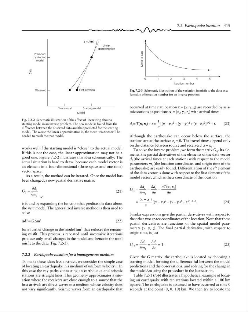
Fig. 7.2-3 Schematic illustration of the variation in misfit to the data as a
function of iteration number for an inverse problem.
7.2 Earthquake location 419
occurred at time t at location x = (x, y, z) are recorded by seismic stations at positions x i = (x i , y i , z i ) with arrival times
d i = T(x, x i ) + t =
1
v
[(x − x i )
2
+ (y − y i )
2
+ (z − z i )
2 ]
1/2
+ t.
(23)
Although the earthquake can occur below the surface, the
stations are at the surface z i = 0. The travel times depend only
on the distance between source and receiver, | x − x i |.
To solve the inverse problem, we form the matrix G ij . Its elements, the partial derivatives of the elements of the data vector
d i (the arrival times at each station) with respect to the model
parameters m j (the location coordinates and origin time of the
earthquake) are easily found. Differentiation of the i th element
of the data vector is done with respect to the first element of the
model vector, which is the x coordinate of the location
G
d
m
d
x
T
x
i
i
i
i
1
1
=
=
=
( , )
∂
∂
∂
∂
∂
∂
x x
=
−
(
)
x x
v
i [(x − x i ) 2 + (y − y i ) 2 + z 2 ] −1/2 .
(24)
Similar expressions give the partial derivatives with respect to
the other two space coordinates of the location. Note that these
partial derivatives are functions of the spatial model parameters (x, y, z). The final partial derivative, with respect to
origin time, is just
G
d
m
d
t
i
i
i
4
4
1
=
=
= .
∂
∂
∂
∂
(25)
Given the G matrix, the earthquake is located by choosing a
starting model, forming the difference ∆d between the model
predictions and the observations, and solving for the change in
the model ∆m using the procedure in the last section.
Table 7.2-1 (top) illustrates a hypothetical example of locating an earthquake with ten stations located within a 100 km
square. The earthquake is assumed to have occurred at time 0
seconds at the point (0, 0, 10) km. We then try to locate the
works well if the starting model is “close” to the actual model.
If this is not the case, the linear approximation may not be a
good one. Figure 7.2-2 illustrates this idea schematically. The
actual situation is hard to draw, because each model vector is
an element in a four-dimensional (three space and one time)
vector space.
As a result, the method can be iterated. Once the model has
been changed, a new partial derivative matrix
G
d
m
ij
i
j
=
∂
∂
m 1
(21)
is found by expanding the function that predicts the data about
the new model. The generalized inverse method is then used to
solve
∆d 1 = G∆m 1
(22)
for a further change in the model ∆m 1 that reduces the remaining misfit. This process is repeated until successive iterations
produce only small changes in the model, and hence in the total
misfit to the data (Fig. 7.2-3).
7.2.2 Earthquake location for a homogeneous medium
To make these ideas less abstract, we consider the simple case
of locating an earthquake in a medium of uniform velocity v. In
this case the ray paths connecting an earthquake and seismic
stations are straight lines. This geometry approximates a situation where the receivers are close enough to a source that the
first arrivals are direct waves in a medium whose velocity does
not vary significantly. Seismic waves from an earthquake that
0
1
2
3
4
5
Iteration number
Data
Predicted
by starting
model
Linear
approximation
Observed
True model
Starting model
Model
First iteration
d = A(m)
Fig. 7.2-2 Schematic illustration of the effect of linearizing about a
starting model in an inverse problem. The new model is found from the
difference between the observed data and that predicted for the starting
model. The worse the linear approximation is, the more iterations will be
needed to reach the true model.
Fig. 7.2-3 Schematic illustration of the variation in misfit to the data as a
function of iteration number for an inverse problem.
7.2 Earthquake location 419
occurred at time t at location x = (x, y, z) are recorded by seismic stations at positions x i = (x i , y i , z i ) with arrival times
d i = T(x, x i ) + t =
1
v
[(x − x i )
2
+ (y − y i )
2
+ (z − z i )
2 ]
1/2
+ t.
(23)
Although the earthquake can occur below the surface, the
stations are at the surface z i = 0. The travel times depend only
on the distance between source and receiver, | x − x i |.
To solve the inverse problem, we form the matrix G ij . Its elements, the partial derivatives of the elements of the data vector
d i (the arrival times at each station) with respect to the model
parameters m j (the location coordinates and origin time of the
earthquake) are easily found. Differentiation of the i th element
of the data vector is done with respect to the first element of the
model vector, which is the x coordinate of the location
G
d
m
d
x
T
x
i
i
i
i
1
1
=
=
=
( , )
∂
∂
∂
∂
∂
∂
x x
=
−
(
)
x x
v
i [(x − x i ) 2 + (y − y i ) 2 + z 2 ] −1/2 .
(24)
Similar expressions give the partial derivatives with respect to
the other two space coordinates of the location. Note that these
partial derivatives are functions of the spatial model parameters (x, y, z). The final partial derivative, with respect to
origin time, is just
G
d
m
d
t
i
i
i
4
4
1
=
=
= .
∂
∂
∂
∂
(25)
Given the G matrix, the earthquake is located by choosing a
starting model, forming the difference ∆d between the model
predictions and the observations, and solving for the change in
the model ∆m using the procedure in the last section.
Table 7.2-1 (top) illustrates a hypothetical example of locating an earthquake with ten stations located within a 100 km
square. The earthquake is assumed to have occurred at time 0
seconds at the point (0, 0, 10) km. We then try to locate the
works well if the starting model is “close” to the actual model.
If this is not the case, the linear approximation may not be a
good one. Figure 7.2-2 illustrates this idea schematically. The
actual situation is hard to draw, because each model vector is
an element in a four-dimensional (three space and one time)
vector space.
As a result, the method can be iterated. Once the model has
been changed, a new partial derivative matrix
G
d
m
ij
i
j
=
∂
∂
m 1
(21)
is found by expanding the function that predicts the data about
the new model. The generalized inverse method is then used to
solve
∆d 1 = G∆m 1
(22)
for a further change in the model ∆m 1 that reduces the remaining misfit. This process is repeated until successive iterations
produce only small changes in the model, and hence in the total
misfit to the data (Fig. 7.2-3).
7.2.2 Earthquake location for a homogeneous medium
To make these ideas less abstract, we consider the simple case
of locating an earthquake in a medium of uniform velocity v. In
this case the ray paths connecting an earthquake and seismic
stations are straight lines. This geometry approximates a situation where the receivers are close enough to a source that the
first arrivals are direct waves in a medium whose velocity does
not vary significantly. Seismic waves from an earthquake that