

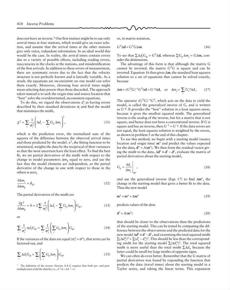
418 Inverse Problems
does not have an inverse. 1 Our first instinct might be to use only
arrival times at four stations, which would give an exact solution, and assume that the arrival times at the other stations
give only extra, redundant information. In an ideal world this
would be the case. In reality, the arrival times contain errors
due to a variety of possible effects, including reading errors,
inaccuracies in the clocks at the stations, and misidentification
of the first arrivals. In addition to these errors of measurement,
there are systematic errors due to the fact that the velocity
structure is not perfectly known and is laterally variable. As a
result, the equations are inconsistent: no one model can solve
them exactly. Moreover, choosing four arrival times might
mean selecting data poorer than those discarded. The approach
taken instead is to seek the origin time and source location that
“best” solve the overdetermined, inconsistent equations.
To do this, we regard the observations d′ i as having errors
described by their standard deviations σ i and find the model
that minimizes the misfit,
χ
σ
2
2
2
1
=
−
⎛
⎝
⎜ ⎜
⎞
⎠
⎟ ⎟
∑
∑
,
i
i
i
i j
j
j
d
G m
∆
∆
(11)
which is the prediction error, the normalized sum of the
squares of the difference between the observed arrival times
and those predicted by the model. x 2 , the fitting function to be
minimized, weights the data by the reciprocal of their variances
so that the most uncertain have the least effect. To find the best
fit, we set partial derivatives of the misfit with respect to the
change in model parameters ∆m k equal to zero, and use the
fact that the model elements are independent, so the partial
derivative of the change in one with respect to those in the
others is zero,
∂
∂
∆
∆
m
m
j
k
jk .
= δ
(12)
The partial derivatives of the misfit are
∂
∂
χ
σ
2
2
0 2
1
∆
∆
∆
m
d
G m G
k
i
i
i
i j
j
j
i k ,
= =
−
⎛
⎝
⎜ ⎜
⎞
⎠
⎟ ⎟
∑
∑
(13)
or
1
1
2
2
σ
σ
i
i
i ik
i
i
ij
j
j
ik
d G
G m G
∑
∑ ∑
=
⎛
⎝
⎜ ⎜
⎞
⎠
⎟ ⎟
∆
∆
.
(14)
If the variances of the data are equal (σ i
2 = σ 2 ), that term can be
factored out, and
∆
∆
d G
G m G
i ik
i
i
ij
j
j
i k
∑
∑ ∑
=
⎛
⎝
⎜ ⎜
⎞
⎠
⎟ ⎟
,
(15)
or, in matrix notation,
G T ∆d = G T G∆m.
(16)
To see that ∑
i
∆d i G ik = G
T
∆d, whereas ∑
j
G ij ∆m j = G∆m, consider the dimensions.
The advantage of this form is that although the matrix G
cannot be inverted, the matrix G
T
G is square and can be
inverted. Equation 16 thus gives ∆m, the standard least squares
solution to a set of equations that cannot be solved exactly,
because
∆m = (G T G) −1 G T ∆d = G −g ∆d, or ∆m j =
G d
ji
g
i
i
−
∑ ∆ . (17)
The operator (G T G) −1 G T , which acts on the data to yield the
model, is called the generalized inverse of G, and is written
as G −g . It provides the “best” solution in a least squares sense,
because it gives the smallest squared misfit. The generalized
inverse is the analog of the inverse, but for a matrix that is not
square, and hence does not have a conventional inverse. If G is
square and has an inverse, then G
−1
= G
−g
. If the data errors are
not equal, the least squares solution is weighted by the errors,
as shown in problem 5 at the end of this chapter.
To use this method, we begin with a starting model (source
location and origin time) m° and predict the values expected
for the data, d° = A(m°). We then form the residual vector giving the misfit to the data, ∆d° ≡ d′ − d°, evaluate the matrix of
partial derivatives about the starting model,
G
d
m
ij
i
j
=
°
,
∂
∂
m
(18)
and use the generalized inverse (Eqn 17) to find ∆m°, the
change in the starting model that gives a better fit to the data.
Thus the new model
m 1 = m° + ∆m°
(19)
predicts values of the data
d 1 = A(m 1 )
(20)
that should be closer to the observations than the predictions
of the starting model. This can be tested by computing the difference between the observations and the predicted data for the
new model ∆d
1
≡ d′ − d
1 , and examining the total squared misfit
∑(∆d i
1 ) 2 = ∑(d i ′ − d i
1 ) 2 . This should be less than the corresponding misfit for the starting model ∑(∆d i
°) 2 . The total squared
misfit is more useful than the total misfit ∑∆d i , because the
latter could be small for large misfits of opposite signs.
We can often do even better. Remember that the G matrix of
partial derivatives was found by expanding the function that
predicts the data (travel times) about the starting model in a
Taylor series, and taking the linear terms. This expansion
1 The definition of the inverse (Section A.4.3) requires that both pre- and postmultiplication yield the identify; i.e., A −1 A = AA −1 = I.
does not have an inverse. 1 Our first instinct might be to use only
arrival times at four stations, which would give an exact solution, and assume that the arrival times at the other stations
give only extra, redundant information. In an ideal world this
would be the case. In reality, the arrival times contain errors
due to a variety of possible effects, including reading errors,
inaccuracies in the clocks at the stations, and misidentification
of the first arrivals. In addition to these errors of measurement,
there are systematic errors due to the fact that the velocity
structure is not perfectly known and is laterally variable. As a
result, the equations are inconsistent: no one model can solve
them exactly. Moreover, choosing four arrival times might
mean selecting data poorer than those discarded. The approach
taken instead is to seek the origin time and source location that
“best” solve the overdetermined, inconsistent equations.
To do this, we regard the observations d′ i as having errors
described by their standard deviations σ i and find the model
that minimizes the misfit,
χ
σ
2
2
2
1
=
−
⎛
⎝
⎜ ⎜
⎞
⎠
⎟ ⎟
∑
∑
,
i
i
i
i j
j
j
d
G m
∆
∆
(11)
which is the prediction error, the normalized sum of the
squares of the difference between the observed arrival times
and those predicted by the model. x 2 , the fitting function to be
minimized, weights the data by the reciprocal of their variances
so that the most uncertain have the least effect. To find the best
fit, we set partial derivatives of the misfit with respect to the
change in model parameters ∆m k equal to zero, and use the
fact that the model elements are independent, so the partial
derivative of the change in one with respect to those in the
others is zero,
∂
∂
∆
∆
m
m
j
k
jk .
= δ
(12)
The partial derivatives of the misfit are
∂
∂
χ
σ
2
2
0 2
1
∆
∆
∆
m
d
G m G
k
i
i
i
i j
j
j
i k ,
= =
−
⎛
⎝
⎜ ⎜
⎞
⎠
⎟ ⎟
∑
∑
(13)
or
1
1
2
2
σ
σ
i
i
i ik
i
i
ij
j
j
ik
d G
G m G
∑
∑ ∑
=
⎛
⎝
⎜ ⎜
⎞
⎠
⎟ ⎟
∆
∆
.
(14)
If the variances of the data are equal (σ i
2 = σ 2 ), that term can be
factored out, and
∆
∆
d G
G m G
i ik
i
i
ij
j
j
i k
∑
∑ ∑
=
⎛
⎝
⎜ ⎜
⎞
⎠
⎟ ⎟
,
(15)
or, in matrix notation,
G T ∆d = G T G∆m.
(16)
To see that ∑
i
∆d i G ik = G
T
∆d, whereas ∑
j
G ij ∆m j = G∆m, consider the dimensions.
The advantage of this form is that although the matrix G
cannot be inverted, the matrix G
T
G is square and can be
inverted. Equation 16 thus gives ∆m, the standard least squares
solution to a set of equations that cannot be solved exactly,
because
∆m = (G T G) −1 G T ∆d = G −g ∆d, or ∆m j =
G d
ji
g
i
i
−
∑ ∆ . (17)
The operator (G T G) −1 G T , which acts on the data to yield the
model, is called the generalized inverse of G, and is written
as G −g . It provides the “best” solution in a least squares sense,
because it gives the smallest squared misfit. The generalized
inverse is the analog of the inverse, but for a matrix that is not
square, and hence does not have a conventional inverse. If G is
square and has an inverse, then G
−1
= G
−g
. If the data errors are
not equal, the least squares solution is weighted by the errors,
as shown in problem 5 at the end of this chapter.
To use this method, we begin with a starting model (source
location and origin time) m° and predict the values expected
for the data, d° = A(m°). We then form the residual vector giving the misfit to the data, ∆d° ≡ d′ − d°, evaluate the matrix of
partial derivatives about the starting model,
G
d
m
ij
i
j
=
°
,
∂
∂
m
(18)
and use the generalized inverse (Eqn 17) to find ∆m°, the
change in the starting model that gives a better fit to the data.
Thus the new model
m 1 = m° + ∆m°
(19)
predicts values of the data
d 1 = A(m 1 )
(20)
that should be closer to the observations than the predictions
of the starting model. This can be tested by computing the difference between the observations and the predicted data for the
new model ∆d
1
≡ d′ − d
1 , and examining the total squared misfit
∑(∆d i
1 ) 2 = ∑(d i ′ − d i
1 ) 2 . This should be less than the corresponding misfit for the starting model ∑(∆d i
°) 2 . The total squared
misfit is more useful than the total misfit ∑∆d i , because the
latter could be small for large misfits of opposite signs.
We can often do even better. Remember that the G matrix of
partial derivatives was found by expanding the function that
predicts the data (travel times) about the starting model in a
Taylor series, and taking the linear terms. This expansion
1 The definition of the inverse (Section A.4.3) requires that both pre- and postmultiplication yield the identify; i.e., A −1 A = AA −1 = I.