

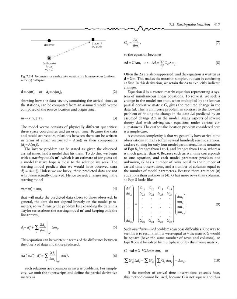
Epicenter
Earthquake
focus
(x, y, z)
Station i
(x i , y i , 0)
G
d
m
ij
i
j
=
,
∂
∂
(7)
so the equation becomes
∆d = G∆m, or ∆d i = G m
ij
j
j
∆
∑
.
(8)
Often the ∆s are also suppressed, and the equation is written as
d = Gm. This makes the notation simpler, but can be confusing
at first. In this derivation, we retain the ∆s to explicitly indicate
changes.
Equation 8 is a vector–matrix equation representing a system of simultaneous linear equations. To solve it, we seek a
change in the model ∆m that, when multiplied by the known
partial derivative matrix G, gives the required change in the
data ∆d. This is an inverse problem, in contrast to the forward
problem of finding the change in the data ∆d predicted by an
assumed change ∆m in the model. Many aspects of inverse
theory deal with solving such equations under various circumstances. The earthquake location problem considered here
is a simple case.
A common complexity is that we generally have arrival time
observations at many (often several hundred) seismic stations,
and are solving for only four model parameters. In the notation
of Eqn 8, j ranges from 1 to 4, and i ranges from 1 to n, where n
is much greater than 4. Because each arrival time corresponds
to one equation, and each model parameter provides one
unknown, G has a number of rows equal to the number of
arrival time observations, and a number of columns equal to
the number of model parameters. Because there are more (n)
equations than unknowns (4), G has more rows than columns,
so Eqn 8 looks like
∆
∆
∆
∆
∆
∆
d
d
d
G
G
G
G
G
G
G
G
G
G
G
G
m
m
n
n
n
n
n
1
2
11
12
13
14
21
22
23
24
1
2
3
4
1
2
⋅
⋅
⋅
⋅
⋅
⎛
⎝
⎜
⎜
⎜
⎜
⎜
⎜
⎜
⎜
⎜
⎞
⎠
⎟
⎟
⎟
⎟
⎟
⎟
⎟
⎟
⎟
=
⋅
⋅
⋅
⋅
⋅
⋅
⋅
⋅
⋅
⋅
⋅
⋅
⋅
⋅
⋅
⋅
⋅
⋅
⋅
⋅
⎛
⎝
⎜
⎜
⎜
⎜
⎜
⎜
⎜
⎜
⎜
⎞
⎠
⎟
⎟
⎟
⎟
⎟
⎟
⎟
⎟
⎟
m m
m
3
4
∆
⎛
⎝
⎜
⎜
⎜
⎜
⎞
⎠
⎟
⎟
⎟
⎟
.
(9)
Such overdetermined problems can pose difficulties. One way to
see this is to recall that if n were equal to 4 the matrix G would
be square (have the same number of rows and columns), so
Eqn 8 could be solved by multiplication by the inverse matrix,
G −1 ∆d = G −1 G∆m = ∆m, or
G d
G
G m
m
ki
i
i
k i
i
ij
j
j
k
−
−
∑
∑
∑
=
⎛
⎝
⎜ ⎜
⎞
⎠
⎟ ⎟
=
1
1
∆
∆
∆ .
(10)
If the number of arrival time observations exceeds four,
this method cannot be used, because G is not square and thus
Fig. 7.2-1 Geometry for earthquake location in a homogeneous (uniform
velocity) halfspace.
d = A(m), or d i = A(m j ),
(2)
showing how the data vector, containing the arrival times at
the stations, can be computed from an assumed model vector
composed of the source location and origin time,
m = (x, y, z, t).
(3)
The model vector consists of physically different quantities:
three space coordinates and an origin time. Because the data
and model are vectors, relations between them can be written
in terms of either vectors (d = A(m)) or their components
(d i = A(m j )).
The inverse problem can be stated as: given the observed
arrival times, find a model that fits them. To do this, we begin
with a starting model m°, which is an estimate of (or guess at)
a model that we hope is close to the solution we seek. The
starting model predicts that we would have observed data
d i
° = A(m j
°). Unless we are lucky, these predicted data are not
what were actually observed. Hence we seek changes ∆m j in the
starting model
m j = m j
° + ∆m j
(4)
that will make the predicted data closer to those observed. In
general, the data do not depend linearly on the model parameters, so we linearize the problem by expanding the data in a
Taylor series about the starting model m° and keeping only the
linear term,
d i ≈ d i
° +
∂
∂
d
m
m
i
j
j
j
∑
°
m
∆ .
(5)
This equation can be written in terms of the difference between
the observed data and those predicted,
∆d i
° ≡ d i
′ − d i
° ≈
∂
∂
d
m
m
i
j
j
j
∑
°
m
°
∆ .
(6)
Such relations are common in inverse problems. For simplicity, we omit the superscripts and define the partial derivative
matrix as
7.2 Earthquake location 417
Earthquake
focus
(x, y, z)
Station i
(x i , y i , 0)
G
d
m
ij
i
j
=
,
∂
∂
(7)
so the equation becomes
∆d = G∆m, or ∆d i = G m
ij
j
j
∆
∑
.
(8)
Often the ∆s are also suppressed, and the equation is written as
d = Gm. This makes the notation simpler, but can be confusing
at first. In this derivation, we retain the ∆s to explicitly indicate
changes.
Equation 8 is a vector–matrix equation representing a system of simultaneous linear equations. To solve it, we seek a
change in the model ∆m that, when multiplied by the known
partial derivative matrix G, gives the required change in the
data ∆d. This is an inverse problem, in contrast to the forward
problem of finding the change in the data ∆d predicted by an
assumed change ∆m in the model. Many aspects of inverse
theory deal with solving such equations under various circumstances. The earthquake location problem considered here
is a simple case.
A common complexity is that we generally have arrival time
observations at many (often several hundred) seismic stations,
and are solving for only four model parameters. In the notation
of Eqn 8, j ranges from 1 to 4, and i ranges from 1 to n, where n
is much greater than 4. Because each arrival time corresponds
to one equation, and each model parameter provides one
unknown, G has a number of rows equal to the number of
arrival time observations, and a number of columns equal to
the number of model parameters. Because there are more (n)
equations than unknowns (4), G has more rows than columns,
so Eqn 8 looks like
∆
∆
∆
∆
∆
∆
d
d
d
G
G
G
G
G
G
G
G
G
G
G
G
m
m
n
n
n
n
n
1
2
11
12
13
14
21
22
23
24
1
2
3
4
1
2
⋅
⋅
⋅
⋅
⋅
⎛
⎝
⎜
⎜
⎜
⎜
⎜
⎜
⎜
⎜
⎜
⎞
⎠
⎟
⎟
⎟
⎟
⎟
⎟
⎟
⎟
⎟
=
⋅
⋅
⋅
⋅
⋅
⋅
⋅
⋅
⋅
⋅
⋅
⋅
⋅
⋅
⋅
⋅
⋅
⋅
⋅
⋅
⎛
⎝
⎜
⎜
⎜
⎜
⎜
⎜
⎜
⎜
⎜
⎞
⎠
⎟
⎟
⎟
⎟
⎟
⎟
⎟
⎟
⎟
m m
m
3
4
∆
⎛
⎝
⎜
⎜
⎜
⎜
⎞
⎠
⎟
⎟
⎟
⎟
.
(9)
Such overdetermined problems can pose difficulties. One way to
see this is to recall that if n were equal to 4 the matrix G would
be square (have the same number of rows and columns), so
Eqn 8 could be solved by multiplication by the inverse matrix,
G −1 ∆d = G −1 G∆m = ∆m, or
G d
G
G m
m
ki
i
i
k i
i
ij
j
j
k
−
−
∑
∑
∑
=
⎛
⎝
⎜ ⎜
⎞
⎠
⎟ ⎟
=
1
1
∆
∆
∆ .
(10)
If the number of arrival time observations exceeds four,
this method cannot be used, because G is not square and thus
Fig. 7.2-1 Geometry for earthquake location in a homogeneous (uniform
velocity) halfspace.
d = A(m), or d i = A(m j ),
(2)
showing how the data vector, containing the arrival times at
the stations, can be computed from an assumed model vector
composed of the source location and origin time,
m = (x, y, z, t).
(3)
The model vector consists of physically different quantities:
three space coordinates and an origin time. Because the data
and model are vectors, relations between them can be written
in terms of either vectors (d = A(m)) or their components
(d i = A(m j )).
The inverse problem can be stated as: given the observed
arrival times, find a model that fits them. To do this, we begin
with a starting model m°, which is an estimate of (or guess at)
a model that we hope is close to the solution we seek. The
starting model predicts that we would have observed data
d i
° = A(m j
°). Unless we are lucky, these predicted data are not
what were actually observed. Hence we seek changes ∆m j in the
starting model
m j = m j
° + ∆m j
(4)
that will make the predicted data closer to those observed. In
general, the data do not depend linearly on the model parameters, so we linearize the problem by expanding the data in a
Taylor series about the starting model m° and keeping only the
linear term,
d i ≈ d i
° +
∂
∂
d
m
m
i
j
j
j
∑
°
m
∆ .
(5)
This equation can be written in terms of the difference between
the observed data and those predicted,
∆d i
° ≡ d i
′ − d i
° ≈
∂
∂
d
m
m
i
j
j
j
∑
°
m
°
∆ .
(6)
Such relations are common in inverse problems. For simplicity, we omit the superscripts and define the partial derivative
matrix as
7.2 Earthquake location 417