

6.6 Seismometers and seismological networks 407
seismogram has the greatest power at low frequencies, and
the acceleration seismogram has the greatest power at high
frequencies. In general, displacements have lower frequencies
than velocities, and velocities have lower frequencies than
accelerations, because integration “smoothes” a signal, whereas
differentiation makes it “rougher.” 6
Figure 6.6-14a illustrates this relation with three different
versions of the same seismogram. If an accelerogram consists of
high-frequency spikes (top), then smoother lower-frequency
velocity (center) and displacement (bottom) traces result from
integrating once and twice. Figure 6.6-14b shows this effect for
a strong-motion seismogram of the 1971 San Fernando earthquake, where the velocity and acceleration records have higher
frequencies than the displacement. It is common in earthquake
engineering to show the response of a structure to ground
motions using a plot that shows the displacement, velocity, and
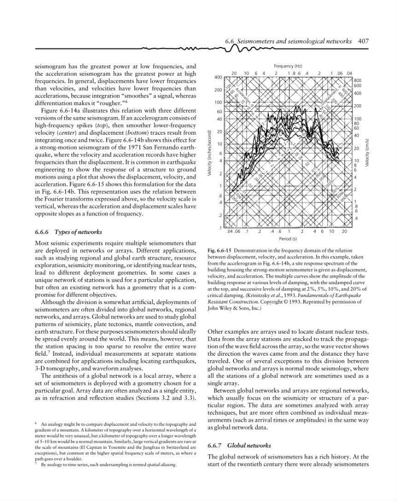
acceleration. Figure 6.6-15 shows this formulation for the data
in Fig. 6.6-14b. This representation uses the relation between
the Fourier transforms expressed above, so the velocity scale is
vertical, whereas the acceleration and displacement scales have
opposite slopes as a function of frequency.
6.6.6 Types of networks
Most seismic experiments require multiple seismometers that
are deployed in networks or arrays. Different applications,
such as studying regional and global earth structure, resource
exploration, seismicity monitoring, or identifying nuclear tests,
lead to different deployment geometries. In some cases a
unique network of stations is used for a particular application,
but often an existing network has a geometry that is a compromise for different objectives.
Although the division is somewhat artificial, deployments of
seismometers are often divided into global networks, regional
networks, and arrays. Global networks are used to study global
patterns of seismicity, plate tectonics, mantle convection, and
earth structure. For these purposes seismometers should ideally
be spread evenly around the world. This means, however, that
the station spacing is too sparse to resolve the entire wave
field. 7 Instead, individual measurements at separate stations
are combined for applications including locating earthquakes,
3-D tomography, and waveform analyses.
The antithesis of a global network is a local array, where a
set of seismometers is deployed with a geometry chosen for a
particular goal. Array data are often analyzed as a single entity,
as in refraction and reflection studies (Sections 3.2 and 3.3).
Velocity (inches/second)
400
200
800
600
Velocity (cm/s)
6 0
1 0 0
4 0
2 0
100
60
40
20
10
6
4
2
1
.6
.4
.2
.1 .04 .06 .1
.2
.4 .6 1
2
4 6 10
20
Period (s)
400
200
100
80
60
40
20
10
8
6
4
2
1
.8
.6
.4
Frequency (Hz)
.04
.06
.1
.2
.4
1
2
4
6
10
20
.8 .6
1 0
6
4
2
1
. 6
. 4
. 2
. 1
. 0 6
. 0 4
. 0 2
. 0 1
. 0 0 6
. 0 0 4
. 0 0 2
. 0 0 1
. 0 0 0 6
. 0 0 0 4
A c c e le
r a t io
n , g
6 0 0
4 0 0
2 0 0
1 0 0
6 0
4 0
2 0
1 0
6
4
2
1
. 6
. 4
. 2
. 1
. 0 6
. 0 4
. 0 2
. 0 1
. 0 0 6
. 0 0 4
D is p la
c e m
e n t , in
Fig. 6.6-15 Demonstration in the frequency domain of the relation
between displacement, velocity, and acceleration. In this example, taken
from the accelerogram in Fig. 6.6-14b, a site response spectrum of the
building housing the strong-motion seismometer is given as displacement,
velocity, and acceleration. The multiple curves show the amplitude of the
building response at various levels of damping, with the undamped curve
at the top, and successive levels of damping at 2%, 5%, 10%, and 20% of
critical damping. (Krinitzsky et al., 1993. Fundamentals of Earthquake
Resistant Construction. Copyright © 1993. Reprinted by permission of
John Wiley & Sons, Inc.)
6 An analogy might be to compare displacement and velocity to the topography and
gradient of a mountain. A kilometer of topography over a horizontal wavelength of a
meter would be very unusual, but a kilometer of topography over a longer wavelength
of 5–10 km would be a normal mountain. Similarly, large vertical gradients are rare at
the scale of mountains (El Capitan in Yosemite and the Jungfrau in Switzerland are
exceptions), but common at the higher spatial frequency scale of meters, as where a
path goes over a boulder.
7 By analogy to time series, such undersampling is termed spatial aliasing.
Other examples are arrays used to locate distant nuclear tests.
Data from the array stations are stacked to track the propagation of the wave field across the array, so the wave vector shows
the direction the waves came from and the distance they have
traveled. One of several exceptions to this division between
global networks and arrays is normal mode seismology, where
all the stations of a global network are sometimes used as a
single array.
Between global networks and arrays are regional networks,
which usually focus on the seismicity or structure of a particular region. The data are sometimes analyzed with array
techniques, but are more often combined as individual measurements (such as arrival times or amplitudes) in the same way
as global network data.
6.6.7 Global networks
The global network of seismometers has a rich history. At the
start of the twentieth century there were already seismometers
seismogram has the greatest power at low frequencies, and
the acceleration seismogram has the greatest power at high
frequencies. In general, displacements have lower frequencies
than velocities, and velocities have lower frequencies than
accelerations, because integration “smoothes” a signal, whereas
differentiation makes it “rougher.” 6
Figure 6.6-14a illustrates this relation with three different
versions of the same seismogram. If an accelerogram consists of
high-frequency spikes (top), then smoother lower-frequency
velocity (center) and displacement (bottom) traces result from
integrating once and twice. Figure 6.6-14b shows this effect for
a strong-motion seismogram of the 1971 San Fernando earthquake, where the velocity and acceleration records have higher
frequencies than the displacement. It is common in earthquake
engineering to show the response of a structure to ground
motions using a plot that shows the displacement, velocity, and
acceleration. Figure 6.6-15 shows this formulation for the data
in Fig. 6.6-14b. This representation uses the relation between
the Fourier transforms expressed above, so the velocity scale is
vertical, whereas the acceleration and displacement scales have
opposite slopes as a function of frequency.
6.6.6 Types of networks
Most seismic experiments require multiple seismometers that
are deployed in networks or arrays. Different applications,
such as studying regional and global earth structure, resource
exploration, seismicity monitoring, or identifying nuclear tests,
lead to different deployment geometries. In some cases a
unique network of stations is used for a particular application,
but often an existing network has a geometry that is a compromise for different objectives.
Although the division is somewhat artificial, deployments of
seismometers are often divided into global networks, regional
networks, and arrays. Global networks are used to study global
patterns of seismicity, plate tectonics, mantle convection, and
earth structure. For these purposes seismometers should ideally
be spread evenly around the world. This means, however, that
the station spacing is too sparse to resolve the entire wave
field. 7 Instead, individual measurements at separate stations
are combined for applications including locating earthquakes,
3-D tomography, and waveform analyses.
The antithesis of a global network is a local array, where a
set of seismometers is deployed with a geometry chosen for a
particular goal. Array data are often analyzed as a single entity,
as in refraction and reflection studies (Sections 3.2 and 3.3).
Velocity (inches/second)
400
200
800
600
Velocity (cm/s)
6 0
1 0 0
4 0
2 0
100
60
40
20
10
6
4
2
1
.6
.4
.2
.1 .04 .06 .1
.2
.4 .6 1
2
4 6 10
20
Period (s)
400
200
100
80
60
40
20
10
8
6
4
2
1
.8
.6
.4
Frequency (Hz)
.04
.06
.1
.2
.4
1
2
4
6
10
20
.8 .6
1 0
6
4
2
1
. 6
. 4
. 2
. 1
. 0 6
. 0 4
. 0 2
. 0 1
. 0 0 6
. 0 0 4
. 0 0 2
. 0 0 1
. 0 0 0 6
. 0 0 0 4
A c c e le
r a t io
n , g
6 0 0
4 0 0
2 0 0
1 0 0
6 0
4 0
2 0
1 0
6
4
2
1
. 6
. 4
. 2
. 1
. 0 6
. 0 4
. 0 2
. 0 1
. 0 0 6
. 0 0 4
D is p la
c e m
e n t , in
Fig. 6.6-15 Demonstration in the frequency domain of the relation
between displacement, velocity, and acceleration. In this example, taken
from the accelerogram in Fig. 6.6-14b, a site response spectrum of the
building housing the strong-motion seismometer is given as displacement,
velocity, and acceleration. The multiple curves show the amplitude of the
building response at various levels of damping, with the undamped curve
at the top, and successive levels of damping at 2%, 5%, 10%, and 20% of
critical damping. (Krinitzsky et al., 1993. Fundamentals of Earthquake
Resistant Construction. Copyright © 1993. Reprinted by permission of
John Wiley & Sons, Inc.)
6 An analogy might be to compare displacement and velocity to the topography and
gradient of a mountain. A kilometer of topography over a horizontal wavelength of a
meter would be very unusual, but a kilometer of topography over a longer wavelength
of 5–10 km would be a normal mountain. Similarly, large vertical gradients are rare at
the scale of mountains (El Capitan in Yosemite and the Jungfrau in Switzerland are
exceptions), but common at the higher spatial frequency scale of meters, as where a
path goes over a boulder.
7 By analogy to time series, such undersampling is termed spatial aliasing.
Other examples are arrays used to locate distant nuclear tests.
Data from the array stations are stacked to track the propagation of the wave field across the array, so the wave vector shows
the direction the waves came from and the distance they have
traveled. One of several exceptions to this division between
global networks and arrays is normal mode seismology, where
all the stations of a global network are sometimes used as a
single array.
Between global networks and arrays are regional networks,
which usually focus on the seismicity or structure of a particular region. The data are sometimes analyzed with array
techniques, but are more often combined as individual measurements (such as arrival times or amplitudes) in the same way
as global network data.
6.6.7 Global networks
The global network of seismometers has a rich history. At the
start of the twentieth century there were already seismometers