

406 Seismograms as Signals
60
Displacement
(cm)
−20
0
20
50
40
30
20
10
0
Time (s)
Velocity
(cm/s)
−30
0
30
Acceleration
(cm/s
2
)
−250
0
250
(b)
Amplitude
(a)
Acceleration
Velocity
Displacement
Time
to filter a seismic signal, so we decide what we seek and what
we will accept as a consequence.
Because the seismogram depends on the instrument response
that is convolved with the ground motion, obtaining the
ground motion requires specifying the frequency response of
the seismometer. This can be done by giving the amplitude
and phase response as a list of the values at each frequency. A
more compact representation gives the frequency response as a
complex fraction like
T i
i
z
i
p
j
j
L
k
k
N
( )
(
)
(
)
.
ω
β
ω
α
ω
=
−
−
=
=
∏
∏
1
1
(10)
The fraction is described by a set of L complex zeros z j at
which the numerator is zero, N complex poles p k at which the
denominator is zero, and the constants β and α. Because the
frequency terms iω are always imaginary and the poles always
contain a real part, the denominator never becomes zero,
avoiding any singular values.
The instrument responses in Fig. 6.6-8 were calculated
from the poles and zeroes of the seismometer responses. For
example, the STS-1 response has three zeroes, all equal to
(0, 0), and four poles, which come as complex conjugates:
(−0.0123, 0.0123), (−0.0123, −0.0123), (−39.1800, 49.1200),
(−39.1800, −49.1200). These poles provide the corner frequencies and determine the sharpness of the corners. Similarly, the
DWWSSN response has five zeroes and 11 poles.
Seismometers record combinations of ground displacement,
velocity, or acceleration, depending upon the application. In a
strong-motion seismometer, the displacements may be greater
than the size of the instrument itself, so accelerations are
measured to keep signals on scale. This makes sense because
accelerations are primarily responsible for damage to structures and so are considered in strong-motion studies. At the
other end of the frequency spectrum, strainmeters are used to
study slow tectonic displacements. In fact, if they measured
accelerations, the signals would be so small as to be unusable.
Most other branches of earthquake seismology fall in between,
using the waves from distant earthquakes, and so use seismometers that record ground velocity.
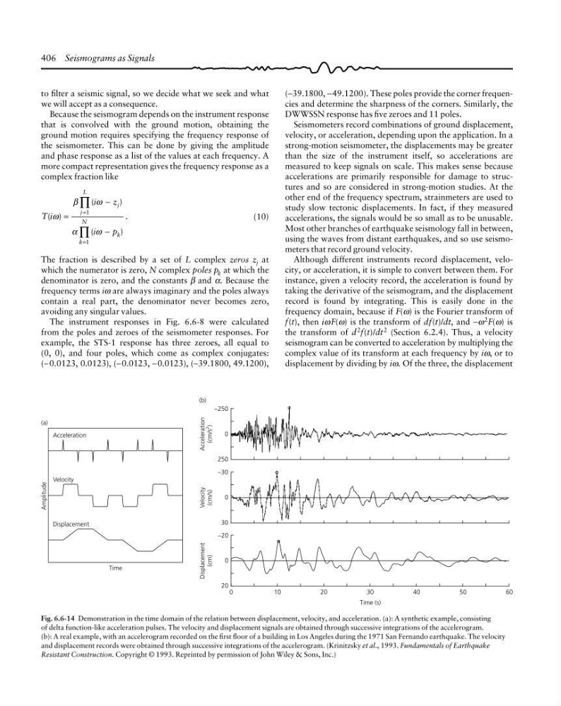
Although different instruments record displacement, velocity, or acceleration, it is simple to convert between them. For
instance, given a velocity record, the acceleration is found by
taking the derivative of the seismogram, and the displacement
record is found by integrating. This is easily done in the
frequency domain, because if F(ω) is the Fourier transform of
f(t), then iωF(ω) is the transform of df(t)/dt, and −ω 2 F(ω) is
the transform of d 2 f(t)/dt 2 (Section 6.2.4). Thus, a velocity
seismogram can be converted to acceleration by multiplying the
complex value of its transform at each frequency by iω, or to
displacement by dividing by iω. Of the three, the displacement
Fig. 6.6-14 Demonstration in the time domain of the relation between displacement, velocity, and acceleration. (a): A synthetic example, consisting
of delta function-like acceleration pulses. The velocity and displacement signals are obtained through successive integrations of the accelerogram.
(b): A real example, with an accelerogram recorded on the first floor of a building in Los Angeles during the 1971 San Fernando earthquake. The velocity
and displacement records were obtained through successive integrations of the accelerogram. (Krinitzsky et al., 1993. Fundamentals of Earthquake
Resistant Construction. Copyright © 1993. Reprinted by permission of John Wiley & Sons, Inc.)
60
Displacement
(cm)
−20
0
20
50
40
30
20
10
0
Time (s)
Velocity
(cm/s)
−30
0
30
Acceleration
(cm/s
2
)
−250
0
250
(b)
Amplitude
(a)
Acceleration
Velocity
Displacement
Time
to filter a seismic signal, so we decide what we seek and what
we will accept as a consequence.
Because the seismogram depends on the instrument response
that is convolved with the ground motion, obtaining the
ground motion requires specifying the frequency response of
the seismometer. This can be done by giving the amplitude
and phase response as a list of the values at each frequency. A
more compact representation gives the frequency response as a
complex fraction like
T i
i
z
i
p
j
j
L
k
k
N
( )
(
)
(
)
.
ω
β
ω
α
ω
=
−
−
=
=
∏
∏
1
1
(10)
The fraction is described by a set of L complex zeros z j at
which the numerator is zero, N complex poles p k at which the
denominator is zero, and the constants β and α. Because the
frequency terms iω are always imaginary and the poles always
contain a real part, the denominator never becomes zero,
avoiding any singular values.
The instrument responses in Fig. 6.6-8 were calculated
from the poles and zeroes of the seismometer responses. For
example, the STS-1 response has three zeroes, all equal to
(0, 0), and four poles, which come as complex conjugates:
(−0.0123, 0.0123), (−0.0123, −0.0123), (−39.1800, 49.1200),
(−39.1800, −49.1200). These poles provide the corner frequencies and determine the sharpness of the corners. Similarly, the
DWWSSN response has five zeroes and 11 poles.
Seismometers record combinations of ground displacement,
velocity, or acceleration, depending upon the application. In a
strong-motion seismometer, the displacements may be greater
than the size of the instrument itself, so accelerations are
measured to keep signals on scale. This makes sense because
accelerations are primarily responsible for damage to structures and so are considered in strong-motion studies. At the
other end of the frequency spectrum, strainmeters are used to
study slow tectonic displacements. In fact, if they measured
accelerations, the signals would be so small as to be unusable.
Most other branches of earthquake seismology fall in between,
using the waves from distant earthquakes, and so use seismometers that record ground velocity.
Although different instruments record displacement, velocity, or acceleration, it is simple to convert between them. For
instance, given a velocity record, the acceleration is found by
taking the derivative of the seismogram, and the displacement
record is found by integrating. This is easily done in the
frequency domain, because if F(ω) is the Fourier transform of
f(t), then iωF(ω) is the transform of df(t)/dt, and −ω 2 F(ω) is
the transform of d 2 f(t)/dt 2 (Section 6.2.4). Thus, a velocity
seismogram can be converted to acceleration by multiplying the
complex value of its transform at each frequency by iω, or to
displacement by dividing by iω. Of the three, the displacement
Fig. 6.6-14 Demonstration in the time domain of the relation between displacement, velocity, and acceleration. (a): A synthetic example, consisting
of delta function-like acceleration pulses. The velocity and displacement signals are obtained through successive integrations of the accelerogram.
(b): A real example, with an accelerogram recorded on the first floor of a building in Los Angeles during the 1971 San Fernando earthquake. The velocity
and displacement records were obtained through successive integrations of the accelerogram. (Krinitzsky et al., 1993. Fundamentals of Earthquake
Resistant Construction. Copyright © 1993. Reprinted by permission of John Wiley & Sons, Inc.)