

402 Seismograms as Signals
Log (sensor response)
a. Pendulum
Amplitude response
Log (trans. response)
c. Transducer
Log (galv. response)
e.
Galvanometer
Log (total response)
g. Total
log g
ω
log s
ω
Log (frequency)
b. Pendulum
d. Transducer
f.
Galvanometer
h. Total
log g
ω
log s
ω
Log (frequency)
Phase response
Phase
Phase
Phase
Phase
0
−π
0
−π
0
−π
0
−π
Recording
drum
Attenuator
Transducer
Galvanometer
V 1
R 1
R 2
V 2
l 2
l 1
Mirror
Light
beam
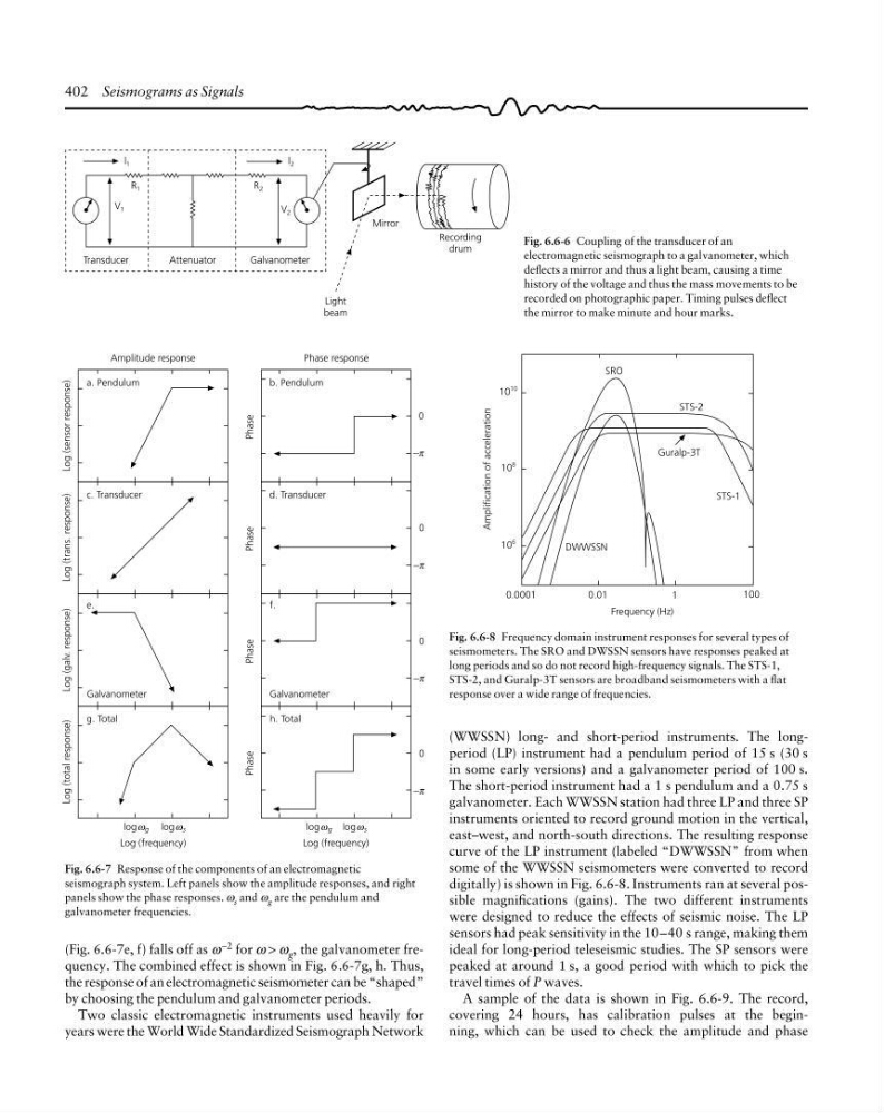
Fig. 6.6-6 Coupling of the transducer of an
electromagnetic seismograph to a galvanometer, which
deflects a mirror and thus a light beam, causing a time
history of the voltage and thus the mass movements to be
recorded on photographic paper. Timing pulses deflect
the mirror to make minute and hour marks.
Fig. 6.6-7 Response of the components of an electromagnetic
seismograph system. Left panels show the amplitude responses, and right
panels show the phase responses. ω s and ω g are the pendulum and
galvanometer frequencies.
(Fig. 6.6-7e, f) falls off as ω
−2 for ω > ω g , the galvanometer frequency. The combined effect is shown in Fig. 6.6-7g, h. Thus,
the response of an electromagnetic seismometer can be “shaped”
by choosing the pendulum and galvanometer periods.
Two classic electromagnetic instruments used heavily for
years were the World Wide Standardized Seismograph Network
Amplification of acceleration
10
10
STS-2
10
8
10
6
SRO
Guralp-3T
STS-1
DWWSSN
0.0001
0.01
1
100
Frequency (Hz)
Fig. 6.6-8 Frequency domain instrument responses for several types of
seismometers. The SRO and DWSSN sensors have responses peaked at
long periods and so do not record high-frequency signals. The STS-1,
STS-2, and Guralp-3T sensors are broadband seismometers with a flat
response over a wide range of frequencies.
(WWSSN) long- and short-period instruments. The longperiod (LP) instrument had a pendulum period of 15 s (30 s
in some early versions) and a galvanometer period of 100 s.
The short-period instrument had a 1 s pendulum and a 0.75 s
galvanometer. Each WWSSN station had three LP and three SP
instruments oriented to record ground motion in the vertical,
east–west, and north-south directions. The resulting response
curve of the LP instrument (labeled “DWWSSN” from when
some of the WWSSN seismometers were converted to record
digitally) is shown in Fig. 6.6-8. Instruments ran at several possible magnifications (gains). The two different instruments
were designed to reduce the effects of seismic noise. The LP
sensors had peak sensitivity in the 10–40 s range, making them
ideal for long-period teleseismic studies. The SP sensors were
peaked at around 1 s, a good period with which to pick the
travel times of P waves.
A sample of the data is shown in Fig. 6.6-9. The record,
covering 24 hours, has calibration pulses at the beginning, which can be used to check the amplitude and phase
Log (sensor response)
a. Pendulum
Amplitude response
Log (trans. response)
c. Transducer
Log (galv. response)
e.
Galvanometer
Log (total response)
g. Total
log g
ω
log s
ω
Log (frequency)
b. Pendulum
d. Transducer
f.
Galvanometer
h. Total
log g
ω
log s
ω
Log (frequency)
Phase response
Phase
Phase
Phase
Phase
0
−π
0
−π
0
−π
0
−π
Recording
drum
Attenuator
Transducer
Galvanometer
V 1
R 1
R 2
V 2
l 2
l 1
Mirror
Light
beam
Fig. 6.6-6 Coupling of the transducer of an
electromagnetic seismograph to a galvanometer, which
deflects a mirror and thus a light beam, causing a time
history of the voltage and thus the mass movements to be
recorded on photographic paper. Timing pulses deflect
the mirror to make minute and hour marks.
Fig. 6.6-7 Response of the components of an electromagnetic
seismograph system. Left panels show the amplitude responses, and right
panels show the phase responses. ω s and ω g are the pendulum and
galvanometer frequencies.
(Fig. 6.6-7e, f) falls off as ω
−2 for ω > ω g , the galvanometer frequency. The combined effect is shown in Fig. 6.6-7g, h. Thus,
the response of an electromagnetic seismometer can be “shaped”
by choosing the pendulum and galvanometer periods.
Two classic electromagnetic instruments used heavily for
years were the World Wide Standardized Seismograph Network
Amplification of acceleration
10
10
STS-2
10
8
10
6
SRO
Guralp-3T
STS-1
DWWSSN
0.0001
0.01
1
100
Frequency (Hz)
Fig. 6.6-8 Frequency domain instrument responses for several types of
seismometers. The SRO and DWSSN sensors have responses peaked at
long periods and so do not record high-frequency signals. The STS-1,
STS-2, and Guralp-3T sensors are broadband seismometers with a flat
response over a wide range of frequencies.
(WWSSN) long- and short-period instruments. The longperiod (LP) instrument had a pendulum period of 15 s (30 s
in some early versions) and a galvanometer period of 100 s.
The short-period instrument had a 1 s pendulum and a 0.75 s
galvanometer. Each WWSSN station had three LP and three SP
instruments oriented to record ground motion in the vertical,
east–west, and north-south directions. The resulting response
curve of the LP instrument (labeled “DWWSSN” from when
some of the WWSSN seismometers were converted to record
digitally) is shown in Fig. 6.6-8. Instruments ran at several possible magnifications (gains). The two different instruments
were designed to reduce the effects of seismic noise. The LP
sensors had peak sensitivity in the 10–40 s range, making them
ideal for long-period teleseismic studies. The SP sensors were
peaked at around 1 s, a good period with which to pick the
travel times of P waves.
A sample of the data is shown in Fig. 6.6-9. The record,
covering 24 hours, has calibration pulses at the beginning, which can be used to check the amplitude and phase