

2 cm
Carson City, Nev. Ewing Duplex Pandutum.
(From photographic copy.)
N
S
E
W
1
0
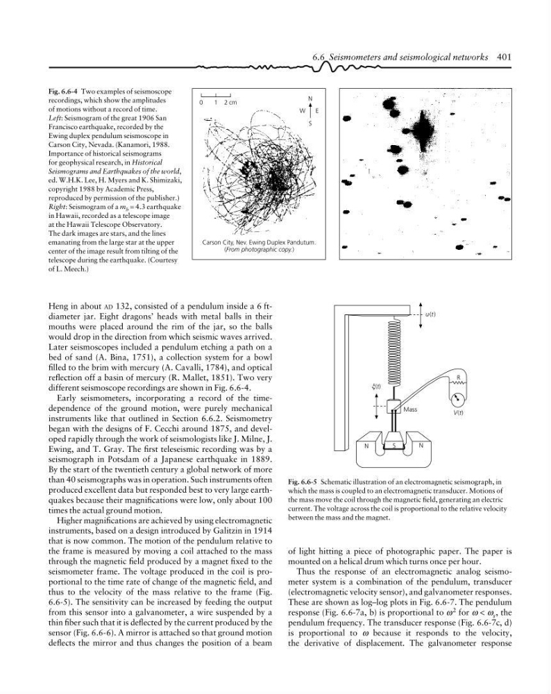
Fig. 6.6-4 Two examples of seismoscope
recordings, which show the amplitudes
of motions without a record of time.
Left: Seismogram of the great 1906 San
Francisco earthquake, recorded by the
Ewing duplex pendulum seismoscope in
Carson City, Nevada. (Kanamori, 1988.
Importance of historical seismograms
for geophysical research, in Historical
Seismograms and Earthquakes of the world,
ed. W.H.K. Lee, H. Myers and K. Shimizaki,
copyright 1988 by Academic Press,
reproduced by permission of the publisher.)
Right: Seismogram of a m b = 4.3 earthquake
in Hawaii, recorded as a telescope image
at the Hawaii Telescope Observatory.
The dark images are stars, and the lines
emanating from the large star at the upper
center of the image result from tilting of the
telescope during the earthquake. (Courtesy
of L. Meech.)
Heng in about AD 132, consisted of a pendulum inside a 6 ftdiameter jar. Eight dragons’ heads with metal balls in their
mouths were placed around the rim of the jar, so the balls
would drop in the direction from which seismic waves arrived.
Later seismoscopes included a pendulum etching a path on a
bed of sand (A. Bina, 1751), a collection system for a bowl
filled to the brim with mercury (A. Cavalli, 1784), and optical
reflection off a basin of mercury (R. Mallet, 1851). Two very
different seismoscope recordings are shown in Fig. 6.6-4.
Early seismometers, incorporating a record of the timedependence of the ground motion, were purely mechanical
instruments like that outlined in Section 6.6.2. Seismometry
began with the designs of F. Cecchi around 1875, and developed rapidly through the work of seismologists like J. Milne, J.
Ewing, and T. Gray. The first teleseismic recording was by a
seismograph in Potsdam of a Japanese earthquake in 1889.
By the start of the twentieth century a global network of more
than 40 seismographs was in operation. Such instruments often
produced excellent data but responded best to very large earthquakes because their magnifications were low, only about 100
times the actual ground motion.
Higher magnifications are achieved by using electromagnetic
instruments, based on a design introduced by Galitzin in 1914
that is now common. The motion of the pendulum relative to
the frame is measured by moving a coil attached to the mass
through the magnetic field produced by a magnet fixed to the
seismometer frame. The voltage produced in the coil is proportional to the time rate of change of the magnetic field, and
thus to the velocity of the mass relative to the frame (Fig.
6.6-5). The sensitivity can be increased by feeding the output
from this sensor into a galvanometer, a wire suspended by a
thin fiber such that it is deflected by the current produced by the
sensor (Fig. 6.6-6). A mirror is attached so that ground motion
deflects the mirror and thus changes the position of a beam
Fig. 6.6-5 Schematic illustration of an electromagnetic seismograph, in
which the mass is coupled to an electromagnetic transducer. Motions of
the mass move the coil through the magnetic field, generating an electric
current. The voltage across the coil is proportional to the relative velocity
between the mass and the magnet.
N
u(t)
V(t)
Mass
N
S
(t)
ξ
R
6.6 Seismometers and seismological networks 401
of light hitting a piece of photographic paper. The paper is
mounted on a helical drum which turns once per hour.
Thus the response of an electromagnetic analog seismometer system is a combination of the pendulum, transducer
(electromagnetic velocity sensor), and galvanometer responses.
These are shown as log–log plots in Fig. 6.6-7. The pendulum
response (Fig. 6.6-7a, b) is proportional to ω 2 for ω < ω s , the
pendulum frequency. The transducer response (Fig. 6.6-7c, d)
is proportional to ω because it responds to the velocity,
the derivative of displacement. The galvanometer response
Carson City, Nev. Ewing Duplex Pandutum.
(From photographic copy.)
N
S
E
W
1
0
Fig. 6.6-4 Two examples of seismoscope
recordings, which show the amplitudes
of motions without a record of time.
Left: Seismogram of the great 1906 San
Francisco earthquake, recorded by the
Ewing duplex pendulum seismoscope in
Carson City, Nevada. (Kanamori, 1988.
Importance of historical seismograms
for geophysical research, in Historical
Seismograms and Earthquakes of the world,
ed. W.H.K. Lee, H. Myers and K. Shimizaki,
copyright 1988 by Academic Press,
reproduced by permission of the publisher.)
Right: Seismogram of a m b = 4.3 earthquake
in Hawaii, recorded as a telescope image
at the Hawaii Telescope Observatory.
The dark images are stars, and the lines
emanating from the large star at the upper
center of the image result from tilting of the
telescope during the earthquake. (Courtesy
of L. Meech.)
Heng in about AD 132, consisted of a pendulum inside a 6 ftdiameter jar. Eight dragons’ heads with metal balls in their
mouths were placed around the rim of the jar, so the balls
would drop in the direction from which seismic waves arrived.
Later seismoscopes included a pendulum etching a path on a
bed of sand (A. Bina, 1751), a collection system for a bowl
filled to the brim with mercury (A. Cavalli, 1784), and optical
reflection off a basin of mercury (R. Mallet, 1851). Two very
different seismoscope recordings are shown in Fig. 6.6-4.
Early seismometers, incorporating a record of the timedependence of the ground motion, were purely mechanical
instruments like that outlined in Section 6.6.2. Seismometry
began with the designs of F. Cecchi around 1875, and developed rapidly through the work of seismologists like J. Milne, J.
Ewing, and T. Gray. The first teleseismic recording was by a
seismograph in Potsdam of a Japanese earthquake in 1889.
By the start of the twentieth century a global network of more
than 40 seismographs was in operation. Such instruments often
produced excellent data but responded best to very large earthquakes because their magnifications were low, only about 100
times the actual ground motion.
Higher magnifications are achieved by using electromagnetic
instruments, based on a design introduced by Galitzin in 1914
that is now common. The motion of the pendulum relative to
the frame is measured by moving a coil attached to the mass
through the magnetic field produced by a magnet fixed to the
seismometer frame. The voltage produced in the coil is proportional to the time rate of change of the magnetic field, and
thus to the velocity of the mass relative to the frame (Fig.
6.6-5). The sensitivity can be increased by feeding the output
from this sensor into a galvanometer, a wire suspended by a
thin fiber such that it is deflected by the current produced by the
sensor (Fig. 6.6-6). A mirror is attached so that ground motion
deflects the mirror and thus changes the position of a beam
Fig. 6.6-5 Schematic illustration of an electromagnetic seismograph, in
which the mass is coupled to an electromagnetic transducer. Motions of
the mass move the coil through the magnetic field, generating an electric
current. The voltage across the coil is proportional to the relative velocity
between the mass and the magnet.
N
u(t)
V(t)
Mass
N
S
(t)
ξ
R
6.6 Seismometers and seismological networks 401
of light hitting a piece of photographic paper. The paper is
mounted on a helical drum which turns once per hour.
Thus the response of an electromagnetic analog seismometer system is a combination of the pendulum, transducer
(electromagnetic velocity sensor), and galvanometer responses.
These are shown as log–log plots in Fig. 6.6-7. The pendulum
response (Fig. 6.6-7a, b) is proportional to ω 2 for ω < ω s , the
pendulum frequency. The transducer response (Fig. 6.6-7c, d)
is proportional to ω because it responds to the velocity,
the derivative of displacement. The galvanometer response