

ω ω
ω ω
h = 0
0.3
0.5
1
2
3
2
1
0
0
1
2
3
0.3
0.5
1
2
h = 0
0
1
2
0 /
0 /
| X( ) |
ω
( )
φ ω
0
π
2
π
If we define ξ(t) − ξ 0 as ξ(t), the displacement relative to the
equilibrium position, Eqn 1 becomes
mQ + dP + kξ = −mü,
(2)
or
Q + 2εP + ω 2
0 ξ = −ü,
(3)
where the single and double dots denote the first and second
time derivatives, ω 0 = k m
/ is the natural frequency of the
undamped system, and the damping is described by ε = d/(2m).
This is a linear differential equation with constant coefficients
that we encountered when we used a damped harmonic oscillator as a model for anelasticity (Section 3.7.5). Thus Eqn 3 is the
inhomogeneous (forcing term) version of Eqn 3.7.8, where the
damping term ε appeared as ω 0 /2Q. To solve it, we assume that
u(t) = e −iωt and ξ(t) = X(ω)e −iωt
(4)
and substitute Eqn 4 into Eqn 3 to yield
X(ω)(−ω
2
− 2εiω + ω
2
0 )e
−iωt
= ω
2 e
−iωt
,
(5)
or
X(ω) = −ω 2 /(ω 2 − ω 2
0 + 2εiω),
(6)
which is the instrument response produced by a ground motion
e iωt .
X(ω) is complex and can be written in terms of the amplitude
and phase responses
X(ω) = | X(ω) |e iφ(ω) ,
(7)
where
| X(ω) | = ω 2 /[(ω 2 − ω 2
0 ) 2 + 4ε 2 ω 2 ] 1/2 ,
(8)
φ(ω) = −tan −1 2
2
0
2
εω
ω
ω
−
+ π.
(9)
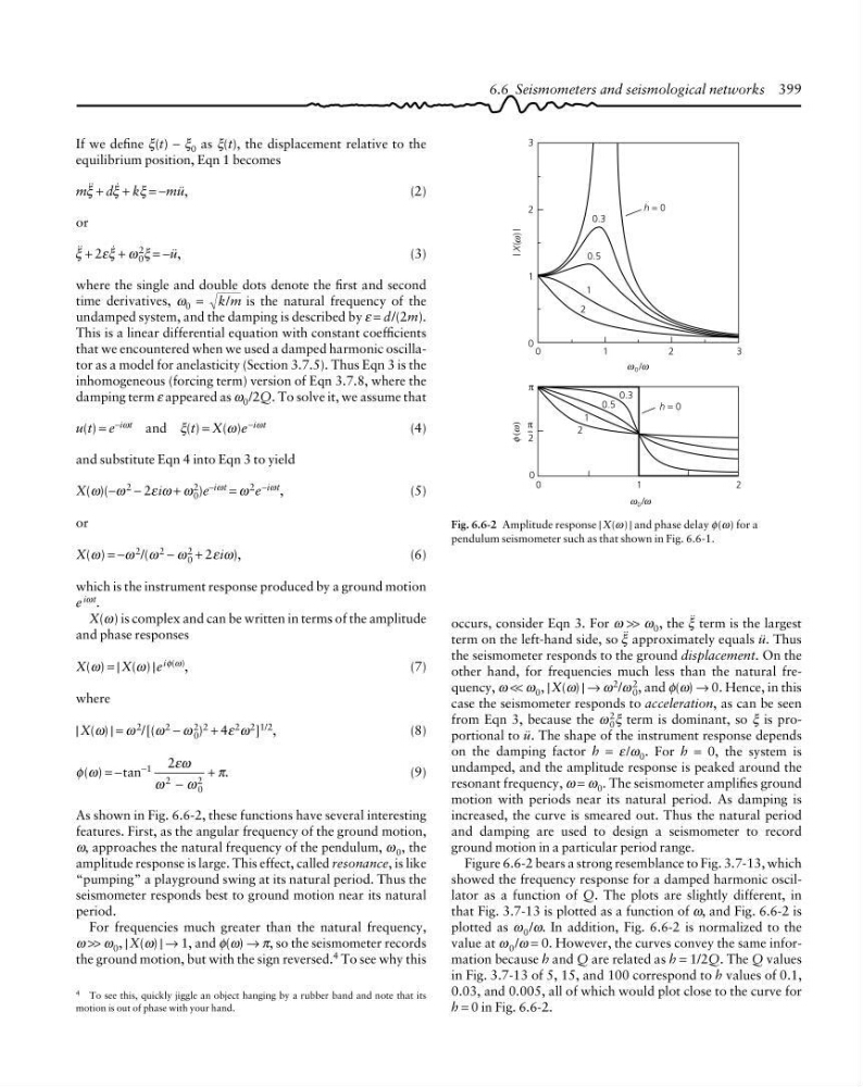
As shown in Fig. 6.6-2, these functions have several interesting
features. First, as the angular frequency of the ground motion,
ω, approaches the natural frequency of the pendulum, ω 0 , the
amplitude response is large. This effect, called resonance, is like
“pumping” a playground swing at its natural period. Thus the
seismometer responds best to ground motion near its natural
period.
For frequencies much greater than the natural frequency,
ω >> ω 0 , | X(ω) | → 1, and φ(ω) → π, so the seismometer records
the ground motion, but with the sign reversed. 4 To see why this
Fig. 6.6-2 Amplitude response | X(ω ) | and phase delay φ(ω) for a
pendulum seismometer such as that shown in Fig. 6.6-1.
4 To see this, quickly jiggle an object hanging by a rubber band and note that its
motion is out of phase with your hand.
6.6 Seismometers and seismological networks 399
occurs, consider Eqn 3. For ω >> ω 0 , the Q term is the largest
term on the left-hand side, so Q approximately equals ü. Thus
the seismometer responds to the ground displacement. On the
other hand, for frequencies much less than the natural frequency, ω << ω 0 , | X(ω) | → ω 2 /ω 2
0 , and φ(ω) → 0. Hence, in this
case the seismometer responds to acceleration, as can be seen
from Eqn 3, because the ω
2
0 ξ term is dominant, so ξ is proportional to ü. The shape of the instrument response depends
on the damping factor h = ε /ω 0 . For h = 0, the system is
undamped, and the amplitude response is peaked around the
resonant frequency, ω = ω 0 . The seismometer amplifies ground
motion with periods near its natural period. As damping is
increased, the curve is smeared out. Thus the natural period
and damping are used to design a seismometer to record
ground motion in a particular period range.
Figure 6.6-2 bears a strong resemblance to Fig. 3.7-13, which
showed the frequency response for a damped harmonic oscillator as a function of Q. The plots are slightly different, in
that Fig. 3.7-13 is plotted as a function of ω, and Fig. 6.6-2 is
plotted as ω 0 /ω. In addition, Fig. 6.6-2 is normalized to the
value at ω 0 /ω = 0. However, the curves convey the same information because h and Q are related as h = 1/2Q. The Q values
in Fig. 3.7-13 of 5, 15, and 100 correspond to h values of 0.1,
0.03, and 0.005, all of which would plot close to the curve for
h = 0 in Fig. 6.6-2.
ω ω
h = 0
0.3
0.5
1
2
3
2
1
0
0
1
2
3
0.3
0.5
1
2
h = 0
0
1
2
0 /
0 /
| X( ) |
ω
( )
φ ω
0
π
2
π
If we define ξ(t) − ξ 0 as ξ(t), the displacement relative to the
equilibrium position, Eqn 1 becomes
mQ + dP + kξ = −mü,
(2)
or
Q + 2εP + ω 2
0 ξ = −ü,
(3)
where the single and double dots denote the first and second
time derivatives, ω 0 = k m
/ is the natural frequency of the
undamped system, and the damping is described by ε = d/(2m).
This is a linear differential equation with constant coefficients
that we encountered when we used a damped harmonic oscillator as a model for anelasticity (Section 3.7.5). Thus Eqn 3 is the
inhomogeneous (forcing term) version of Eqn 3.7.8, where the
damping term ε appeared as ω 0 /2Q. To solve it, we assume that
u(t) = e −iωt and ξ(t) = X(ω)e −iωt
(4)
and substitute Eqn 4 into Eqn 3 to yield
X(ω)(−ω
2
− 2εiω + ω
2
0 )e
−iωt
= ω
2 e
−iωt
,
(5)
or
X(ω) = −ω 2 /(ω 2 − ω 2
0 + 2εiω),
(6)
which is the instrument response produced by a ground motion
e iωt .
X(ω) is complex and can be written in terms of the amplitude
and phase responses
X(ω) = | X(ω) |e iφ(ω) ,
(7)
where
| X(ω) | = ω 2 /[(ω 2 − ω 2
0 ) 2 + 4ε 2 ω 2 ] 1/2 ,
(8)
φ(ω) = −tan −1 2
2
0
2
εω
ω
ω
−
+ π.
(9)
As shown in Fig. 6.6-2, these functions have several interesting
features. First, as the angular frequency of the ground motion,
ω, approaches the natural frequency of the pendulum, ω 0 , the
amplitude response is large. This effect, called resonance, is like
“pumping” a playground swing at its natural period. Thus the
seismometer responds best to ground motion near its natural
period.
For frequencies much greater than the natural frequency,
ω >> ω 0 , | X(ω) | → 1, and φ(ω) → π, so the seismometer records
the ground motion, but with the sign reversed. 4 To see why this
Fig. 6.6-2 Amplitude response | X(ω ) | and phase delay φ(ω) for a
pendulum seismometer such as that shown in Fig. 6.6-1.
4 To see this, quickly jiggle an object hanging by a rubber band and note that its
motion is out of phase with your hand.
6.6 Seismometers and seismological networks 399
occurs, consider Eqn 3. For ω >> ω 0 , the Q term is the largest
term on the left-hand side, so Q approximately equals ü. Thus
the seismometer responds to the ground displacement. On the
other hand, for frequencies much less than the natural frequency, ω << ω 0 , | X(ω) | → ω 2 /ω 2
0 , and φ(ω) → 0. Hence, in this
case the seismometer responds to acceleration, as can be seen
from Eqn 3, because the ω
2
0 ξ term is dominant, so ξ is proportional to ü. The shape of the instrument response depends
on the damping factor h = ε /ω 0 . For h = 0, the system is
undamped, and the amplitude response is peaked around the
resonant frequency, ω = ω 0 . The seismometer amplifies ground
motion with periods near its natural period. As damping is
increased, the curve is smeared out. Thus the natural period
and damping are used to design a seismometer to record
ground motion in a particular period range.
Figure 6.6-2 bears a strong resemblance to Fig. 3.7-13, which
showed the frequency response for a damped harmonic oscillator as a function of Q. The plots are slightly different, in
that Fig. 3.7-13 is plotted as a function of ω, and Fig. 6.6-2 is
plotted as ω 0 /ω. In addition, Fig. 6.6-2 is normalized to the
value at ω 0 /ω = 0. However, the curves convey the same information because h and Q are related as h = 1/2Q. The Q values
in Fig. 3.7-13 of 5, 15, and 100 correspond to h values of 0.1,
0.03, and 0.005, all of which would plot close to the curve for
h = 0 in Fig. 6.6-2.