

396 Seismograms as Signals
Slowness (s /km)
Zero-slowness streak →
0.10
0
100
200
Time (s)
Slant stack of April 3, 1985, Bonin earthquake
Upper mantle
arrivals
Slant stack artifacts
PP
sP
pP
P
−0.01
Background
noise level
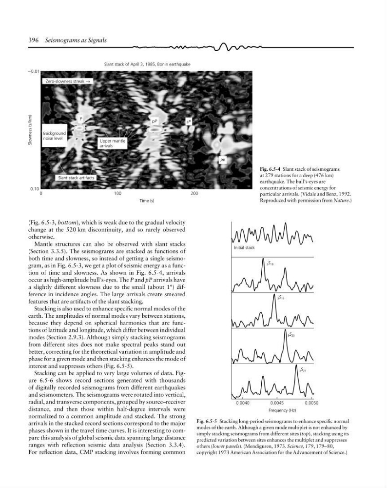
Fig. 6.5-4 Slant stack of seismograms
at 279 stations for a deep (476 km)
earthquake. The bull’s-eyes are
concentrations of seismic energy for
particular arrivals. (Vidale and Benz, 1992.
Reproduced with permission from Nature.)
(Fig. 6.5-3, bottom), which is weak due to the gradual velocity
change at the 520 km discontinuity, and so rarely observed
otherwise.
Mantle structures can also be observed with slant stacks
(Section 3.3.5). The seismograms are stacked as functions of
both time and slowness, so instead of getting a single seismogram, as in Fig. 6.5-3, we get a plot of seismic energy as a function of time and slowness. As shown in Fig. 6.5-4, arrivals
occur as high-amplitude bull’s-eyes. The P and pP arrivals have
a slightly different slowness due to the small (about 1°) difference in incidence angles. The large arrivals create smeared
features that are artifacts of the slant stacking.
Stacking is also used to enhance specific normal modes of the
earth. The amplitudes of normal modes vary between stations,
because they depend on spherical harmonics that are functions of latitude and longitude, which differ between individual
modes (Section 2.9.3). Although simply stacking seismograms
from different sites does not make spectral peaks stand out
better, correcting for the theoretical variation in amplitude and
phase for a given mode and then stacking enhances the mode of
interest and suppresses others (Fig. 6.5-5).
Stacking can be applied to very large volumes of data. Figure 6.5-6 shows record sections generated with thousands
of digitally recorded seismograms from different earthquakes
and seismometers. The seismograms were rotated into vertical,
radial, and transverse components, grouped by source–receiver
distance, and then those within half-degree intervals were
normalized to a common amplitude and stacked. The strong
arrivals in the stacked record sections correspond to the major
phases shown in the travel time curves. It is interesting to compare this analysis of global seismic data spanning large distance
ranges with reflection seismic data analysis (Section 3.3.4).
For reflection data, CMP stacking involves forming common
Fig. 6.5-5 Stacking long-period seismograms to enhance specific normal
modes of the earth. Although a given mode multiplet is not enhanced by
simply stacking seismograms from different sites (top), stacking using its
predicted variation between sites enhances the multiplet and suppresses
others (lower panels). (Mendiguren, 1973. Science, 179, 179–80,
copyright 1973 American Association for the Advancement of Science.)
Initial stack
3 S 18
3 S 19
3 S 20
0.0040
0.0045
0.0050
Frequency (Hz)
3 S 21
Slowness (s /km)
Zero-slowness streak →
0.10
0
100
200
Time (s)
Slant stack of April 3, 1985, Bonin earthquake
Upper mantle
arrivals
Slant stack artifacts
PP
sP
pP
P
−0.01
Background
noise level
Fig. 6.5-4 Slant stack of seismograms
at 279 stations for a deep (476 km)
earthquake. The bull’s-eyes are
concentrations of seismic energy for
particular arrivals. (Vidale and Benz, 1992.
Reproduced with permission from Nature.)
(Fig. 6.5-3, bottom), which is weak due to the gradual velocity
change at the 520 km discontinuity, and so rarely observed
otherwise.
Mantle structures can also be observed with slant stacks
(Section 3.3.5). The seismograms are stacked as functions of
both time and slowness, so instead of getting a single seismogram, as in Fig. 6.5-3, we get a plot of seismic energy as a function of time and slowness. As shown in Fig. 6.5-4, arrivals
occur as high-amplitude bull’s-eyes. The P and pP arrivals have
a slightly different slowness due to the small (about 1°) difference in incidence angles. The large arrivals create smeared
features that are artifacts of the slant stacking.
Stacking is also used to enhance specific normal modes of the
earth. The amplitudes of normal modes vary between stations,
because they depend on spherical harmonics that are functions of latitude and longitude, which differ between individual
modes (Section 2.9.3). Although simply stacking seismograms
from different sites does not make spectral peaks stand out
better, correcting for the theoretical variation in amplitude and
phase for a given mode and then stacking enhances the mode of
interest and suppresses others (Fig. 6.5-5).
Stacking can be applied to very large volumes of data. Figure 6.5-6 shows record sections generated with thousands
of digitally recorded seismograms from different earthquakes
and seismometers. The seismograms were rotated into vertical,
radial, and transverse components, grouped by source–receiver
distance, and then those within half-degree intervals were
normalized to a common amplitude and stacked. The strong
arrivals in the stacked record sections correspond to the major
phases shown in the travel time curves. It is interesting to compare this analysis of global seismic data spanning large distance
ranges with reflection seismic data analysis (Section 3.3.4).
For reflection data, CMP stacking involves forming common
Fig. 6.5-5 Stacking long-period seismograms to enhance specific normal
modes of the earth. Although a given mode multiplet is not enhanced by
simply stacking seismograms from different sites (top), stacking using its
predicted variation between sites enhances the multiplet and suppresses
others (lower panels). (Mendiguren, 1973. Science, 179, 179–80,
copyright 1973 American Association for the Advancement of Science.)
Initial stack
3 S 18
3 S 19
3 S 20
0.0040
0.0045
0.0050
Frequency (Hz)
3 S 21