

1.0
0.8
0.6
0.4
0.2
0.0
−0.2
−0.4
−0.6
S 660 S
S 410 S
amp = 10x
SS
SS Precursor Stack
Time (min.)
−6
−5
−4
−3
−2
−1
0
1
2
Fit to S 410 S and S 660 S
660
410
stacked data
scaled SS
−6
−5
−4
−3
−2
−1
0.04
0.03
0.02
0.01
0.00
−0.01
−0.02
−6
−5
−4
−3
−2
−1
0.04
0.03
0.02
0.01
0.00
− 0.01
− 0.02
520
Stripped of 410 and 660
Time (min.)
This simple Gaussian model is widely used in analyzing data.
We assume that each measurement includes the quantity of
interest and some noise, defined as the portion of the signal that
is not of interest. The noise thus reflects both true errors
of measurement and processes not under consideration, all of
which are assumed to be uncorrelated between measurements.
To the extent that these assumptions are valid, stacking data
will improve the signal. The random, uncorrelated noise idea
often seems to be a good approximation. However, if noise is
correlated between measurements, as can occur if the measurement equipment is biased or an “error” source is otherwise
common to the measurements, the desired noise reduction
will be less. For instance, the structure under a seismometer is
studied by means of receiver functions that are derived using
the radial and vertical components (Fig. 6.3-7), assuming that
the noise on each is uncorrelated. However, noise due to
microseismic activity (Section 6.6.3) will be correlated between
components and hence can yield spurious layering.
6.5.2 Stacking examples
A simple stacking approach is to add seismograms at nearby
stations, assuming that they contain a common signal of interest
plus “noise” that differs between stations. The noise includes
differences in the response of the seismometers and differences
in the seismograms generated by the interaction between the
upcoming waves and the crustal structure under each seismometer. If the seismometers and crustal structure are similar
enough, stacking seismograms should reduce the noise and
yield a better representation of the signal of interest than the
individual seismograms.
An extension of this idea is used for seismograms at different
places or times. If we know theoretically how the signal of
interest varies as a function of position or time, we can correct
the data to a common position or time and stack them. For
example, in CMP stacking of reflection seismic data, traces
with a common midpoint are shifted by a time corresponding
to the travel time curve of a reflection and then stacked (Section
3.3.4). The reflected arrivals are in phase and thus enhanced,
whereas other arrivals with different travel time curves are out
of phase and thus suppressed. Although the undesired arrivals
are not random noise, they are reduced relative to the reflected
arrivals. Random noise in the data is also reduced.
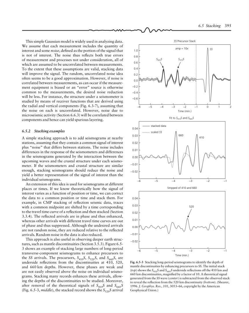
This approach is also useful in observing deeper earth structures, such as mantle discontinuities (Section 3.5.3). Figure 6.53 shows an example of stacking large numbers of long-period
transverse-component seismograms to enhance precursors to
the SS arrivals. The precursors, S 410 S, S 520 S, and S 660 S, are
underside reflections from the discontinuities at 410, 520,
and 660 km depths. However, these phases are weak and
are not easily observed above the noise on individual seismograms. Stacking many records enhances these arrivals, allowing the depths of the discontinuities to be studied. Moreover,
after removal of the theoretical signals of S 410 S and S 660 S
(Fig. 6.5-3, middle), the stacked record shows the S 520 S arrival
Fig. 6.5-3 Stacking long-period seismograms to identify the depth of
mantle discontinuities by enhancing precursors to SS. The initial stack
(top) shows the S 410 S and S 660 S underside reflections off the 410 km and
660 km discontinuities, magnified by a factor of 10. A theoretical signal
generated from the SS wave (center) is subtracted from the observed stack
to reveal the reflection from the 520 km discontinuity (bottom). (Shearer,
1996. J. Geophys. Res., 101, 3053–66, copyright by the American
Geophysical Union.)
6.5 Stacking 395
0.8
0.6
0.4
0.2
0.0
−0.2
−0.4
−0.6
S 660 S
S 410 S
amp = 10x
SS
SS Precursor Stack
Time (min.)
−6
−5
−4
−3
−2
−1
0
1
2
Fit to S 410 S and S 660 S
660
410
stacked data
scaled SS
−6
−5
−4
−3
−2
−1
0.04
0.03
0.02
0.01
0.00
−0.01
−0.02
−6
−5
−4
−3
−2
−1
0.04
0.03
0.02
0.01
0.00
− 0.01
− 0.02
520
Stripped of 410 and 660
Time (min.)
This simple Gaussian model is widely used in analyzing data.
We assume that each measurement includes the quantity of
interest and some noise, defined as the portion of the signal that
is not of interest. The noise thus reflects both true errors
of measurement and processes not under consideration, all of
which are assumed to be uncorrelated between measurements.
To the extent that these assumptions are valid, stacking data
will improve the signal. The random, uncorrelated noise idea
often seems to be a good approximation. However, if noise is
correlated between measurements, as can occur if the measurement equipment is biased or an “error” source is otherwise
common to the measurements, the desired noise reduction
will be less. For instance, the structure under a seismometer is
studied by means of receiver functions that are derived using
the radial and vertical components (Fig. 6.3-7), assuming that
the noise on each is uncorrelated. However, noise due to
microseismic activity (Section 6.6.3) will be correlated between
components and hence can yield spurious layering.
6.5.2 Stacking examples
A simple stacking approach is to add seismograms at nearby
stations, assuming that they contain a common signal of interest
plus “noise” that differs between stations. The noise includes
differences in the response of the seismometers and differences
in the seismograms generated by the interaction between the
upcoming waves and the crustal structure under each seismometer. If the seismometers and crustal structure are similar
enough, stacking seismograms should reduce the noise and
yield a better representation of the signal of interest than the
individual seismograms.
An extension of this idea is used for seismograms at different
places or times. If we know theoretically how the signal of
interest varies as a function of position or time, we can correct
the data to a common position or time and stack them. For
example, in CMP stacking of reflection seismic data, traces
with a common midpoint are shifted by a time corresponding
to the travel time curve of a reflection and then stacked (Section
3.3.4). The reflected arrivals are in phase and thus enhanced,
whereas other arrivals with different travel time curves are out
of phase and thus suppressed. Although the undesired arrivals
are not random noise, they are reduced relative to the reflected
arrivals. Random noise in the data is also reduced.
This approach is also useful in observing deeper earth structures, such as mantle discontinuities (Section 3.5.3). Figure 6.53 shows an example of stacking large numbers of long-period
transverse-component seismograms to enhance precursors to
the SS arrivals. The precursors, S 410 S, S 520 S, and S 660 S, are
underside reflections from the discontinuities at 410, 520,
and 660 km depths. However, these phases are weak and
are not easily observed above the noise on individual seismograms. Stacking many records enhances these arrivals, allowing the depths of the discontinuities to be studied. Moreover,
after removal of the theoretical signals of S 410 S and S 660 S
(Fig. 6.5-3, middle), the stacked record shows the S 520 S arrival
Fig. 6.5-3 Stacking long-period seismograms to identify the depth of
mantle discontinuities by enhancing precursors to SS. The initial stack
(top) shows the S 410 S and S 660 S underside reflections off the 410 km and
660 km discontinuities, magnified by a factor of 10. A theoretical signal
generated from the SS wave (center) is subtracted from the observed stack
to reveal the reflection from the 520 km discontinuity (bottom). (Shearer,
1996. J. Geophys. Res., 101, 3053–66, copyright by the American
Geophysical Union.)
6.5 Stacking 395