

394 Seismograms as Signals
′ = −0.11
N = 100
−2
0
2
N = 1000
′ = −0.04
−2
0
2
N = 10,000
−2
0
2
z
µ
µ
′ = −0.01
µ
To simplify this expression, we use the variances of each variable about its mean
σ 2
u = lim
N
i
N
N
→∞
=
∑
1
1
(u i − I) 2 and σ 2
v = lim
N
i
N
N
→∞
=
∑
1
1
(v i − J) 2
(16)
and the covariances that describe how fluctuations between
variables are correlated:
σ 2
uv = lim
N
i
N
N
→∞
=
∑
1
1
(u i − I)(v i − J).
(17)
Substituting Eqns 16 and 17 into Eqn 15 gives
σ
σ
σ
σ
z
u
v
u v
z
u
z
v
z
u
z
v
2
2
2
2
2
2
2
. . .
. . .
=
⎛
⎝
⎜
⎞
⎠
⎟ +
⎛
⎝
⎜
⎞
⎠
⎟ +
+
⎛
⎝
⎜
⎞
⎠
⎟
⎛
⎝
⎜
⎞
⎠
⎟ +
∂
∂
∂
∂
∂
∂
∂
∂
(18)
This relation, called the propagation of errors equation, illustrates that the extent to which the uncertainty in each variable
contributes to the uncertainty in a function depends on the
partial derivative of the function with respect to that variable.
We often assume that the variations in the different variables
are uncorrelated (which is not always the case), so we set the
covariances equal to zero, and simplify the variance of z to
σ
σ
σ
z
u
v
z
u
z
v
2
2
2
2
2
. . .
=
⎛
⎝
⎜
⎞
⎠
⎟ +
⎛
⎝
⎜
⎞
⎠
⎟ +
∂
∂
∂
∂
(19)
This result is a general one that we have already mentioned
in the context of estimating the uncertainty of geodetic rates
(Eqn 4.5.8) and earthquake source parameters (Eqn 4.6.23).
In the specific application here, we consider the mean to be a
function of the observations,
z = µ′ =
1
1
N i
N
=
∑ x i ,
(20)
so the error propagation equation can be used with (u, v, . . . )
= x i . Assuming that the variables are independent, so their
errors are uncorrelated, we get
σ
σ
µ
σ
σ
µ′
∂ ′
∂
∂
∂
2
1
2
2
1
2
1
2
2
2
1
1
1
.
=
⎛
⎝
⎜
⎞
⎠
⎟ =
⎛
⎝
⎜
⎜
⎞
⎠
⎟
⎟
=
=
=
=
=
∑
∑
∑
∑
i
N
x
i
i
N
x
i
i
i
N
x
i
N
i
i
i
x
N x
x
N
(21)
If all the observations have equal uncertainties (σ 2
x i
= σ 2 ), then
σ
2
µ′ = σ
2
/N.
(22)
Thus the variance of the mean is 1/N times the variance of
the individual measurements. Hence making N measurements
reduces the standard deviation of the mean by 1/ N. This is the
basic idea behind stacking; averaging multiple measurements
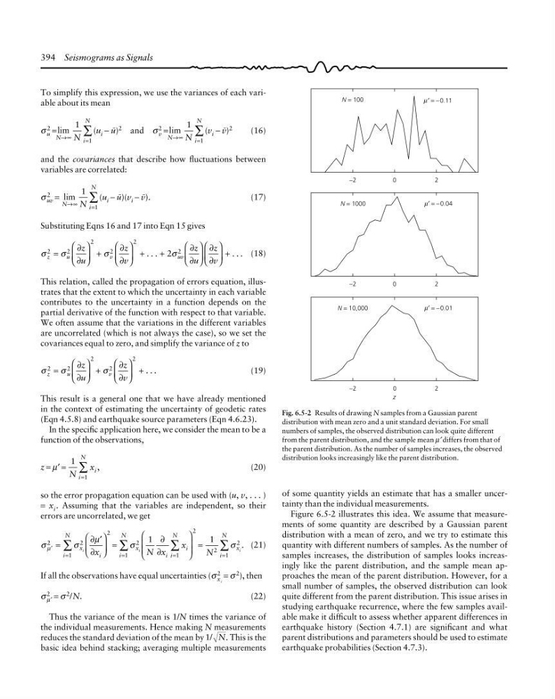
Fig. 6.5-2 Results of drawing N samples from a Gaussian parent
distribution with mean zero and a unit standard deviation. For small
numbers of samples, the observed distribution can look quite different
from the parent distribution, and the sample mean µ′ differs from that of
the parent distribution. As the number of samples increases, the observed
distribution looks increasingly like the parent distribution.
of some quantity yields an estimate that has a smaller uncertainty than the individual measurements.
Figure 6.5-2 illustrates this idea. We assume that measurements of some quantity are described by a Gaussian parent
distribution with a mean of zero, and we try to estimate this
quantity with different numbers of samples. As the number of
samples increases, the distribution of samples looks increasingly like the parent distribution, and the sample mean approaches the mean of the parent distribution. However, for a
small number of samples, the observed distribution can look
quite different from the parent distribution. This issue arises in
studying earthquake recurrence, where the few samples available make it difficult to assess whether apparent differences in
earthquake history (Section 4.7.1) are significant and what
parent distributions and parameters should be used to estimate
earthquake probabilities (Section 4.7.3).
′ = −0.11
N = 100
−2
0
2
N = 1000
′ = −0.04
−2
0
2
N = 10,000
−2
0
2
z
µ
µ
′ = −0.01
µ
To simplify this expression, we use the variances of each variable about its mean
σ 2
u = lim
N
i
N
N
→∞
=
∑
1
1
(u i − I) 2 and σ 2
v = lim
N
i
N
N
→∞
=
∑
1
1
(v i − J) 2
(16)
and the covariances that describe how fluctuations between
variables are correlated:
σ 2
uv = lim
N
i
N
N
→∞
=
∑
1
1
(u i − I)(v i − J).
(17)
Substituting Eqns 16 and 17 into Eqn 15 gives
σ
σ
σ
σ
z
u
v
u v
z
u
z
v
z
u
z
v
2
2
2
2
2
2
2
. . .
. . .
=
⎛
⎝
⎜
⎞
⎠
⎟ +
⎛
⎝
⎜
⎞
⎠
⎟ +
+
⎛
⎝
⎜
⎞
⎠
⎟
⎛
⎝
⎜
⎞
⎠
⎟ +
∂
∂
∂
∂
∂
∂
∂
∂
(18)
This relation, called the propagation of errors equation, illustrates that the extent to which the uncertainty in each variable
contributes to the uncertainty in a function depends on the
partial derivative of the function with respect to that variable.
We often assume that the variations in the different variables
are uncorrelated (which is not always the case), so we set the
covariances equal to zero, and simplify the variance of z to
σ
σ
σ
z
u
v
z
u
z
v
2
2
2
2
2
. . .
=
⎛
⎝
⎜
⎞
⎠
⎟ +
⎛
⎝
⎜
⎞
⎠
⎟ +
∂
∂
∂
∂
(19)
This result is a general one that we have already mentioned
in the context of estimating the uncertainty of geodetic rates
(Eqn 4.5.8) and earthquake source parameters (Eqn 4.6.23).
In the specific application here, we consider the mean to be a
function of the observations,
z = µ′ =
1
1
N i
N
=
∑ x i ,
(20)
so the error propagation equation can be used with (u, v, . . . )
= x i . Assuming that the variables are independent, so their
errors are uncorrelated, we get
σ
σ
µ
σ
σ
µ′
∂ ′
∂
∂
∂
2
1
2
2
1
2
1
2
2
2
1
1
1
.
=
⎛
⎝
⎜
⎞
⎠
⎟ =
⎛
⎝
⎜
⎜
⎞
⎠
⎟
⎟
=
=
=
=
=
∑
∑
∑
∑
i
N
x
i
i
N
x
i
i
i
N
x
i
N
i
i
i
x
N x
x
N
(21)
If all the observations have equal uncertainties (σ 2
x i
= σ 2 ), then
σ
2
µ′ = σ
2
/N.
(22)
Thus the variance of the mean is 1/N times the variance of
the individual measurements. Hence making N measurements
reduces the standard deviation of the mean by 1/ N. This is the
basic idea behind stacking; averaging multiple measurements
Fig. 6.5-2 Results of drawing N samples from a Gaussian parent
distribution with mean zero and a unit standard deviation. For small
numbers of samples, the observed distribution can look quite different
from the parent distribution, and the sample mean µ′ differs from that of
the parent distribution. As the number of samples increases, the observed
distribution looks increasingly like the parent distribution.
of some quantity yields an estimate that has a smaller uncertainty than the individual measurements.
Figure 6.5-2 illustrates this idea. We assume that measurements of some quantity are described by a Gaussian parent
distribution with a mean of zero, and we try to estimate this
quantity with different numbers of samples. As the number of
samples increases, the distribution of samples looks increasingly like the parent distribution, and the sample mean approaches the mean of the parent distribution. However, for a
small number of samples, the observed distribution can look
quite different from the parent distribution. This issue arises in
studying earthquake recurrence, where the few samples available make it difficult to assess whether apparent differences in
earthquake history (Section 4.7.1) are significant and what
parent distributions and parameters should be used to estimate
earthquake probabilities (Section 4.7.3).