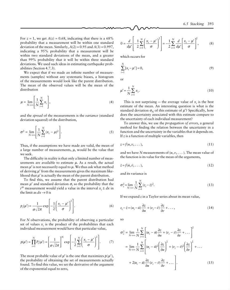
For z = 1, we get A(z) = 0.68, indicating that there is a 68%
probability that a measurement will be within one standard
deviation of the mean. Similarly, A(2) = 0.95 and A(3) = 0.997,
indicating a 95% probability that a measurement will be
within two standard deviations of the mean, and a greater
than 99% probability that it will be within three standard
deviations. We used such ideas in estimating earthquake probabilities (Section 4.7.3).
We expect that if we made an infinite number of measurements (samples) without any systematic biases, a histogram
of the measurements would look like the parent distribution.
The mean of the observed values will be the mean of the
distribution
µ lim
,
=
⎡
⎣
⎢
⎢
⎤
⎦
⎥
⎥
→∞
=
∑
N
i
i
N
N
x
1
1
(4)
and the spread of the measurements is the variance (standard
deviation squared) of the distribution,
σ
µ
2
2
1
1
=
−
⎡
⎣
⎢
⎢
⎤
⎦
⎥
⎥
→∞
=
∑
lim
(
) .
N
i
i
N
N
x
(5)
Thus, if the assumptions we have made are valid, the mean of
a large number of measurements, µ, would be the value that
we seek.
The difficulty in reality is that only a limited number of measurements are available to estimate µ. As a result, the actual
mean µ′ is not necessarily equal to µ. We thus ask what method
of deriving µ′ from the measurements gives the maximum likelihood that µ′ is actually the mean of the parent distribution.
To find this, we assume that the parent distribution had
mean µ′ and standard deviation σ, so the probability that the
i th measurement would yield a value in the interval x i ± dx in
the limit as dx → 0 is
p i (µ′) =
1
2
1
2
2
σ π
µ
σ
exp
.
−
− ′
⎛
⎝
⎜
⎞
⎠
⎟
⎡
⎣
⎢
⎢
⎢
⎤
⎦
⎥
⎥
⎥
x i
(6)
For N observations, the probability of observing a particular
set of values x i is the product of the probabilities that each
individual measurement would have that particular value,
p
P
x
i
i
N
N
i
i
N
( )
( )
exp
.
µ
µ
σ π
µ
σ
′
′
=
=
⎡
⎣
⎢
⎢
⎤
⎦
⎥
⎥
−
− ′
⎛
⎝
⎜
⎞
⎠
⎟
⎡
⎣
⎢
⎢
⎢
⎤
⎦
⎥
⎥
⎥
=
=
∏
∑
1
2
1
1
2
1
2
(7)
The most probable value of µ′ is the one that maximizes p(µ′),
the probability of obtaining the set of measurements actually
found. To find this value, we set the derivative of the argument
of the exponential equal to zero,
0
1
2
1
2
2
1
2
1
,
=
−
−
⎛
⎝
⎜
⎞
⎠
⎟
⎡
⎣
⎢
⎢
⎢
⎤
⎦
⎥
⎥
⎥
= −
−
⎡
⎣
⎢
⎢
⎤
⎦
⎥
⎥
=
=
∑
∑
d
d
x
d
d
x
i
i
N
i
i
N
µ
µ
σ
µ
µ
σ
′
′
′
′
(8)
which occurs for
i
N
=
∑
1
[x i − µ′] = 0,
(9)
or
µ′ =
1
1
N i
N
=
∑ x i .
(10)
This is not surprising a the average value of x i is the best
estimate of the mean. An interesting question is what is the
standard deviation σ N of this estimate of µ′? Specifically, how
does the uncertainty associated with this estimate compare to
the uncertainty of each individual measurement?
To answer this, we use the propagation of errors, a general
method for finding the relation between the uncertainty in a
function and the uncertainty in the variables that it depends on.
If z is a function of multiple variables, then
z = f(u, v, . . . ),
(11)
and we have N measurements of (u, v, . . . ). The mean value of
the function is its value for the mean of the arguments,
K = f(I, J, . . . ),
(12)
and its variance is
σ 2
z = lim
N
i
N
N
→∞
=
∑
1
1
(z i − K) 2 .
(13)
If we expand z in a Taylor series about its mean value,
z i − K = (u i − I)
∂
∂
z
u
+ (v i − J)
∂
∂
z
v
+ . . . ,
(14)
so
σ z N
i
N
i
i
N
u
z
u
v
z
v
2
1
2
1
lim
(
)
(
)
. . .
=
−
+
−
+
⎡
⎣
⎢
⎢
⎤
⎦
⎥
⎥
→∞
=
∑
I
J
∂
∂
∂
∂
=
−
⎛
⎝
⎜
⎞
⎠
⎟ +
−
⎛
⎝
⎜
⎞
⎠
⎟ +
⎡
⎣
⎢
⎢
⎢
→∞
=
∑
lim
(
)
(
)
. . .
N
i
N
i
i
N
u
z
u
v
z
v
1
1
2
2
2
2
I
J
∂
∂
∂
∂
+
−
−
+
⎤
⎦
⎥
⎥
⎥
(
) (
)
. . . .
i
i
u
z
u
v
z
v
2
I
J
∂
∂
∂
∂
(15)
6.5 Stacking 393