

392 Seismograms as Signals
A further complexity is that different methods can measure
related but not identical entities: the earthquake depth ranges
inferred from travel times, waveform modeling, aftershock
locations, and geodesy differ somewhat, because each measures related but not identical quantities.
Most discussions of these issues focus on random errors
because they are easy to estimate from the scatter of measurements. However, it is worth bearing in mind that systematic
errors not included in these error estimates can be more
significant, as discussed in Section 1.1.2. Systematic errors can
come about in surprising ways and have subtle and crucial
effects. For example, we have noted that velocity heterogeneities can perturb ray paths and thus bias earthquake focal
mechanisms (Section 3.7.3); attenuation variations can bias
estimates of the yields of nuclear explosions (Section 1.2.8);
errors in the paleomagnetic time scale can bias estimates of
plate motions (Section 5.2.2); and effects including an undetected earthquake can change estimates of earthquake recurrence from paleoseismology (Section 1.2.5). Systematic biases
are difficult to detect, but sometimes are identified from discrepancies between different approaches. For example, the
discrepancy between earth models derived from body waves
and those from normal modes suggests physical dispersion due
to anelasticity (Section 3.7.8), and the discrepancy between
oceanic Love and Rayleigh wave velocities points toward
anisotropy (Section 3.6.5). Hence, when data are discordant,
as in the differences in earthquake frequency–magnitude
relations derived from seismological and paleoseismic data
(Section 4.7.1), systematic bias is one possible cause.
In this section, we develop some general ideas about errors
and consider some examples. Our focus is one of the most
useful methods for improving estimates from seismological
data: stacking, or taking multiple measurements and averaging
them. We do this either by averaging measurements such as
travel times from different seismograms, or by adding many
seismograms and then estimating parameters. This process has
two effects. First, it improves precision by reducing the effects
of random noise in the data. Second, if the data are averaged
in specific ways, the precision, and perhaps accuracy, can be
improved by suppressing some features of the data and thus
enhancing desired features.
6.5.1 Random errors
We seek to estimate a quantity x from multiple measurements,
each of which gives a value x i due to noise and the limitations
of the measurements. With enough measurements, a pattern
generally emerges in which the values x i are distributed about a
value x′. If we neglect systematic errors of measurement, we
can estimate the value of x from the measured values x i and say
something about how this estimate is related to the unknown
true value of x.
For this purpose we view the measured values x i as random
samples from a parent distribution described by the probability
density function p(x) that gives the probability of observing
a certain value. For example, in Section 4.7.3 we treated the
occurrence of earthquakes as samples from a parent distribution of recurrence times. That example illustrated that in most
applications it is not clear what the most suitable parent distribution is. It is common to assume that the parent distribution is a
Gaussian distribution, also called the “normal distribution,”
because it often describes the frequencies at which very different phenomena occur. A famous result called the central limit
theorem shows that this is because a sum of random numbers
approaches a Gaussian distribution even if the random
numbers are derived from other probability distributions.
For a Gaussian distribution, the probability that the i th
measurement would yield a value in the interval x i ± dx, in the
limit as dx → 0, is
p x
x
dx
i
i
( )
exp
.
=
−
−
⎛
⎝
⎜
⎞
⎠
⎟
⎡
⎣
⎢
⎢
⎢
⎤
⎦
⎥
⎥
⎥
1
2
1
2
2
σ π
µ
σ
(1)
The distribution is thus characterized by two parameters: the
mean, µ, and the standard deviation, σ. The most probable
measurement is the mean value, and values on either side of it
are less likely the further from the mean they are. The distribution is often written as a function of the normalized variable
z = (x − µ)/σ,
p(z) =
1
2π
exp [−z 2 /2]dz.
(2)
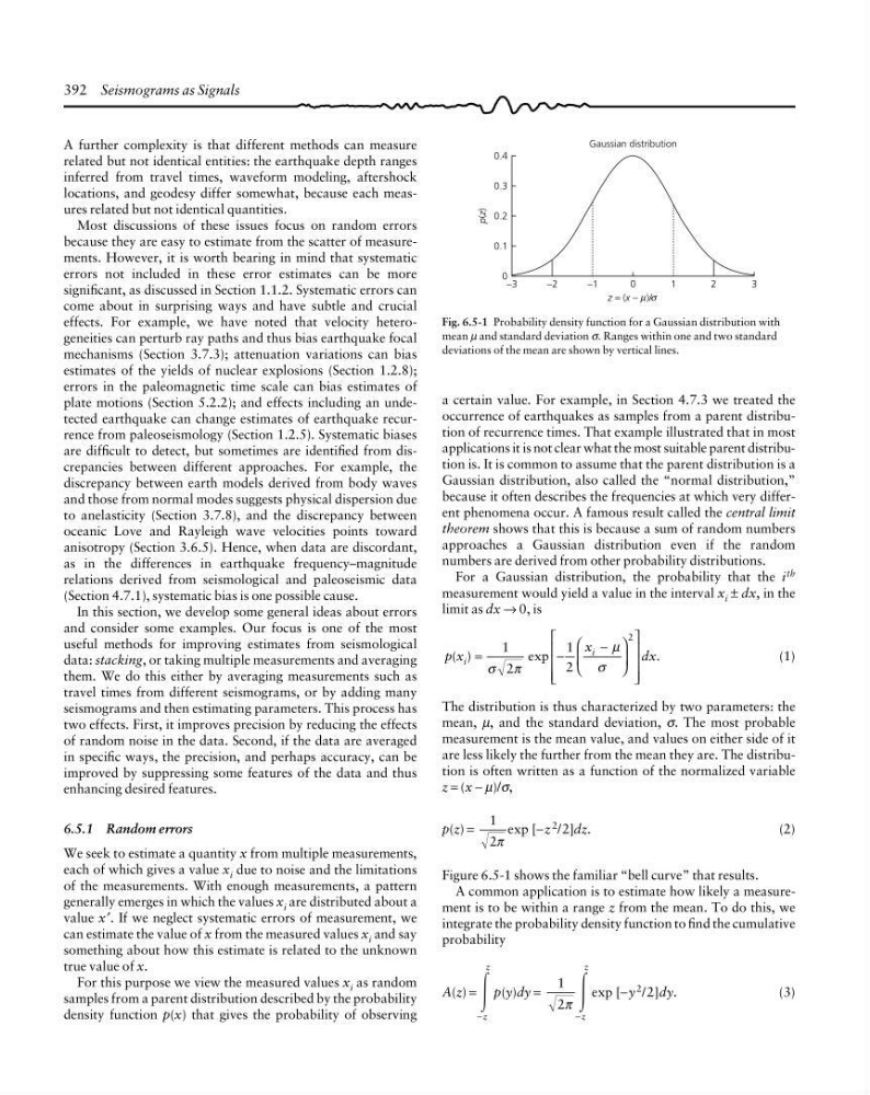
Figure 6.5-1 shows the familiar “bell curve” that results.
A common application is to estimate how likely a measurement is to be within a range z from the mean. To do this, we
integrate the probability density function to find the cumulative
probability
A(z) =
Ύ
− z
z
p(y)dy =
1
2π Ύ
− z
z
exp [−y
2 /2]dy.
(3)
p(z)
0.4
0.3
0.2
0.1
0
3
−3
z = (x − )/
−2
−1
0
1
2
Gaussian distribution
σ
µ
Fig. 6.5-1 Probability density function for a Gaussian distribution with
mean µ and standard deviation σ. Ranges within one and two standard
deviations of the mean are shown by vertical lines.
A further complexity is that different methods can measure
related but not identical entities: the earthquake depth ranges
inferred from travel times, waveform modeling, aftershock
locations, and geodesy differ somewhat, because each measures related but not identical quantities.
Most discussions of these issues focus on random errors
because they are easy to estimate from the scatter of measurements. However, it is worth bearing in mind that systematic
errors not included in these error estimates can be more
significant, as discussed in Section 1.1.2. Systematic errors can
come about in surprising ways and have subtle and crucial
effects. For example, we have noted that velocity heterogeneities can perturb ray paths and thus bias earthquake focal
mechanisms (Section 3.7.3); attenuation variations can bias
estimates of the yields of nuclear explosions (Section 1.2.8);
errors in the paleomagnetic time scale can bias estimates of
plate motions (Section 5.2.2); and effects including an undetected earthquake can change estimates of earthquake recurrence from paleoseismology (Section 1.2.5). Systematic biases
are difficult to detect, but sometimes are identified from discrepancies between different approaches. For example, the
discrepancy between earth models derived from body waves
and those from normal modes suggests physical dispersion due
to anelasticity (Section 3.7.8), and the discrepancy between
oceanic Love and Rayleigh wave velocities points toward
anisotropy (Section 3.6.5). Hence, when data are discordant,
as in the differences in earthquake frequency–magnitude
relations derived from seismological and paleoseismic data
(Section 4.7.1), systematic bias is one possible cause.
In this section, we develop some general ideas about errors
and consider some examples. Our focus is one of the most
useful methods for improving estimates from seismological
data: stacking, or taking multiple measurements and averaging
them. We do this either by averaging measurements such as
travel times from different seismograms, or by adding many
seismograms and then estimating parameters. This process has
two effects. First, it improves precision by reducing the effects
of random noise in the data. Second, if the data are averaged
in specific ways, the precision, and perhaps accuracy, can be
improved by suppressing some features of the data and thus
enhancing desired features.
6.5.1 Random errors
We seek to estimate a quantity x from multiple measurements,
each of which gives a value x i due to noise and the limitations
of the measurements. With enough measurements, a pattern
generally emerges in which the values x i are distributed about a
value x′. If we neglect systematic errors of measurement, we
can estimate the value of x from the measured values x i and say
something about how this estimate is related to the unknown
true value of x.
For this purpose we view the measured values x i as random
samples from a parent distribution described by the probability
density function p(x) that gives the probability of observing
a certain value. For example, in Section 4.7.3 we treated the
occurrence of earthquakes as samples from a parent distribution of recurrence times. That example illustrated that in most
applications it is not clear what the most suitable parent distribution is. It is common to assume that the parent distribution is a
Gaussian distribution, also called the “normal distribution,”
because it often describes the frequencies at which very different phenomena occur. A famous result called the central limit
theorem shows that this is because a sum of random numbers
approaches a Gaussian distribution even if the random
numbers are derived from other probability distributions.
For a Gaussian distribution, the probability that the i th
measurement would yield a value in the interval x i ± dx, in the
limit as dx → 0, is
p x
x
dx
i
i
( )
exp
.
=
−
−
⎛
⎝
⎜
⎞
⎠
⎟
⎡
⎣
⎢
⎢
⎢
⎤
⎦
⎥
⎥
⎥
1
2
1
2
2
σ π
µ
σ
(1)
The distribution is thus characterized by two parameters: the
mean, µ, and the standard deviation, σ. The most probable
measurement is the mean value, and values on either side of it
are less likely the further from the mean they are. The distribution is often written as a function of the normalized variable
z = (x − µ)/σ,
p(z) =
1
2π
exp [−z 2 /2]dz.
(2)
Figure 6.5-1 shows the familiar “bell curve” that results.
A common application is to estimate how likely a measurement is to be within a range z from the mean. To do this, we
integrate the probability density function to find the cumulative
probability
A(z) =
Ύ
− z
z
p(y)dy =
1
2π Ύ
− z
z
exp [−y
2 /2]dy.
(3)
p(z)
0.4
0.3
0.2
0.1
0
3
−3
z = (x − )/
−2
−1
0
1
2
Gaussian distribution
σ
µ
Fig. 6.5-1 Probability density function for a Gaussian distribution with
mean µ and standard deviation σ. Ranges within one and two standard
deviations of the mean are shown by vertical lines.