

Because x(m) and f(n) have different lengths, the points in
the two transforms would correspond to different angular
frequencies. To avoid this, the two time series are extended
with zeroes at their ends, so that their lengths equal the same
power of 2.
A further point to bear in mind is that the time series corresponding to the convolution is longer than either of the two
series that are convolved. If the number of points in the DFT
is less than this length, a wraparound phenomenon similar
to aliasing occurs when we invert the transform, due to the
periodicity resulting from the sampled transform. The two time
series thus need to be extended to a length at least that of their
convolution before their DFTs are taken.
6.5 Stacking
Seismology uses data to estimate quantities that describe the
earth and seismic sources. Ideally these estimates are both
accurate and precise. Accuracy measures the deviation of the
estimate from its true value, whereas precision measures
the repeatability of individual estimates. Hence the accuracy
depends on systematic errors that bias groups of estimates,
whereas the precision depends on random errors that affect
individual estimates. Estimates can be precise but inaccurate,
or accurate but imprecise. For example, an estimate of an
earthquake’s location depends on the quality of the travel time
data used and the accuracy of the velocity model. High-quality
travel time data, together with an incorrect velocity model, can
yield a location that is precise in that the data are well fit and
so imply small uncertainty, but inaccurate in that the resulting
location is not where the earthquake occurred. In such a case
the true uncertainty exceeds the formal uncertainty inferred
from how well the model fits the data. Conversely, an accurate
velocity model and poor travel time data can give a location
that is accurate in that it is close to where the earthquake
occurred, but imprecise in that the location has a large uncertainty and there are large misfits to the data.
Approaches to improving the accuracy and precision of
estimates are often couched in terms of measuring a quantity
like the length of a table. Accuracy is improved by using different measuring tools, ideally calibrated against each other.
Precision is improved by making multiple measurements,
ideally by different people. We follow such approaches for the
earth when possible, but face additional complexities. For
example, an earthquake is a nonrepeatable experiment, so we
cannot make additional measurements. We can use different
techniques, but still face difficulties. A case in point is that
estimates of an earthquake’s depth from travel times and
waveform modeling are only partially independent. Both can
be biased similarly by incorrect assumptions about the nearsource velocity, but the travel times are independent of the
assumed source mechanism, and the waveform modeling
(which depends on relative arrival times) would not be biased
by an error in the absolute timing of individual seismograms.
y(2) = x(0)f(2) + x(1)f(1) + x(2)f(0)
x(3) x(2) x(1) x(0)
f(0) f(1) f(2)
y(1) = x(0)f(1) + x(1)f(0)
x(3) x(2) x(1) x(0)
f(0) f(1) f(2)
y(0) = x(0)f(0)
x(3) x(2) x(1) x(0)
f(0) f(1) f(2)
y(3) = x(1)f(2) + x(2)f(1) + x(3)f(0)
x(3) x(2) x(1) x(0)
y(4) = x(2)f(2) + x(3)f(1)
y(5) = x(3)f(2)
f(0) f(1) f(2)
f(0) f(1) f(2)
x(3) x(2) x(1) x(0)
f(0) f(1) f(2)
x(3) x(2) x(1) x(0)
Reverse
Slide
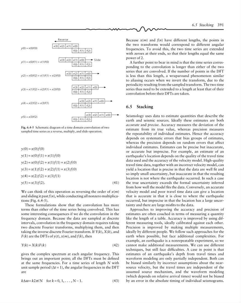
Fig. 6.4-5 Schematic diagram of a time domain convolution of two
sampled time series as a reverse, multiply, and slide operation.
y(0) = x(0)f(0)
y(1) = x(0)f(1) + x(1)f(0)
y(2) = x(0)f(2) + x(1)f(1) + x(2)f(0)
y(3) = x(1)f(2) + x(2)f(1) + x(3)f(0)
y(4) = x(2)f(2) + x(3)f(1)
y(5) = x(3)f(2).
(41)
We can think of this operation as reversing the order of x(m)
and sliding it past f(n), while conducting all nonzero multiplications (Fig. 6.4-5).
These formulations show that the convolution has more
terms than either of the time series being convolved. This has
some interesting consequences if we do the convolution in the
frequency domain. Because the data are sampled at discrete
intervals, convolution in the frequency domain requires taking
two discrete Fourier transforms, multiplying them, and then
taking the inverse discrete Fourier transform. If Y(k), X(k), and
F(k) are the DFTs of y(t), x(m), and f(k), then
Y(k) = X(k)F(k)
(42)
gives the complex spectrum at each angular frequency. This
brings out an important point; all the DFTs must be defined
at the same frequencies. For a time series of length N with
unit sample period (∆t = 1), the angular frequencies in the DFT
are
k∆ω = k2π /N for k = 0, 1, . . . , N − 1.
(43)
6.5 Stacking 391
the two transforms would correspond to different angular
frequencies. To avoid this, the two time series are extended
with zeroes at their ends, so that their lengths equal the same
power of 2.
A further point to bear in mind is that the time series corresponding to the convolution is longer than either of the two
series that are convolved. If the number of points in the DFT
is less than this length, a wraparound phenomenon similar
to aliasing occurs when we invert the transform, due to the
periodicity resulting from the sampled transform. The two time
series thus need to be extended to a length at least that of their
convolution before their DFTs are taken.
6.5 Stacking
Seismology uses data to estimate quantities that describe the
earth and seismic sources. Ideally these estimates are both
accurate and precise. Accuracy measures the deviation of the
estimate from its true value, whereas precision measures
the repeatability of individual estimates. Hence the accuracy
depends on systematic errors that bias groups of estimates,
whereas the precision depends on random errors that affect
individual estimates. Estimates can be precise but inaccurate,
or accurate but imprecise. For example, an estimate of an
earthquake’s location depends on the quality of the travel time
data used and the accuracy of the velocity model. High-quality
travel time data, together with an incorrect velocity model, can
yield a location that is precise in that the data are well fit and
so imply small uncertainty, but inaccurate in that the resulting
location is not where the earthquake occurred. In such a case
the true uncertainty exceeds the formal uncertainty inferred
from how well the model fits the data. Conversely, an accurate
velocity model and poor travel time data can give a location
that is accurate in that it is close to where the earthquake
occurred, but imprecise in that the location has a large uncertainty and there are large misfits to the data.
Approaches to improving the accuracy and precision of
estimates are often couched in terms of measuring a quantity
like the length of a table. Accuracy is improved by using different measuring tools, ideally calibrated against each other.
Precision is improved by making multiple measurements,
ideally by different people. We follow such approaches for the
earth when possible, but face additional complexities. For
example, an earthquake is a nonrepeatable experiment, so we
cannot make additional measurements. We can use different
techniques, but still face difficulties. A case in point is that
estimates of an earthquake’s depth from travel times and
waveform modeling are only partially independent. Both can
be biased similarly by incorrect assumptions about the nearsource velocity, but the travel times are independent of the
assumed source mechanism, and the waveform modeling
(which depends on relative arrival times) would not be biased
by an error in the absolute timing of individual seismograms.
y(2) = x(0)f(2) + x(1)f(1) + x(2)f(0)
x(3) x(2) x(1) x(0)
f(0) f(1) f(2)
y(1) = x(0)f(1) + x(1)f(0)
x(3) x(2) x(1) x(0)
f(0) f(1) f(2)
y(0) = x(0)f(0)
x(3) x(2) x(1) x(0)
f(0) f(1) f(2)
y(3) = x(1)f(2) + x(2)f(1) + x(3)f(0)
x(3) x(2) x(1) x(0)
y(4) = x(2)f(2) + x(3)f(1)
y(5) = x(3)f(2)
f(0) f(1) f(2)
f(0) f(1) f(2)
x(3) x(2) x(1) x(0)
f(0) f(1) f(2)
x(3) x(2) x(1) x(0)
Reverse
Slide
Fig. 6.4-5 Schematic diagram of a time domain convolution of two
sampled time series as a reverse, multiply, and slide operation.
y(0) = x(0)f(0)
y(1) = x(0)f(1) + x(1)f(0)
y(2) = x(0)f(2) + x(1)f(1) + x(2)f(0)
y(3) = x(1)f(2) + x(2)f(1) + x(3)f(0)
y(4) = x(2)f(2) + x(3)f(1)
y(5) = x(3)f(2).
(41)
We can think of this operation as reversing the order of x(m)
and sliding it past f(n), while conducting all nonzero multiplications (Fig. 6.4-5).
These formulations show that the convolution has more
terms than either of the time series being convolved. This has
some interesting consequences if we do the convolution in the
frequency domain. Because the data are sampled at discrete
intervals, convolution in the frequency domain requires taking
two discrete Fourier transforms, multiplying them, and then
taking the inverse discrete Fourier transform. If Y(k), X(k), and
F(k) are the DFTs of y(t), x(m), and f(k), then
Y(k) = X(k)F(k)
(42)
gives the complex spectrum at each angular frequency. This
brings out an important point; all the DFTs must be defined
at the same frequencies. For a time series of length N with
unit sample period (∆t = 1), the angular frequencies in the DFT
are
k∆ω = k2π /N for k = 0, 1, . . . , N − 1.
(43)
6.5 Stacking 391