

Actual signal
Aliased signal
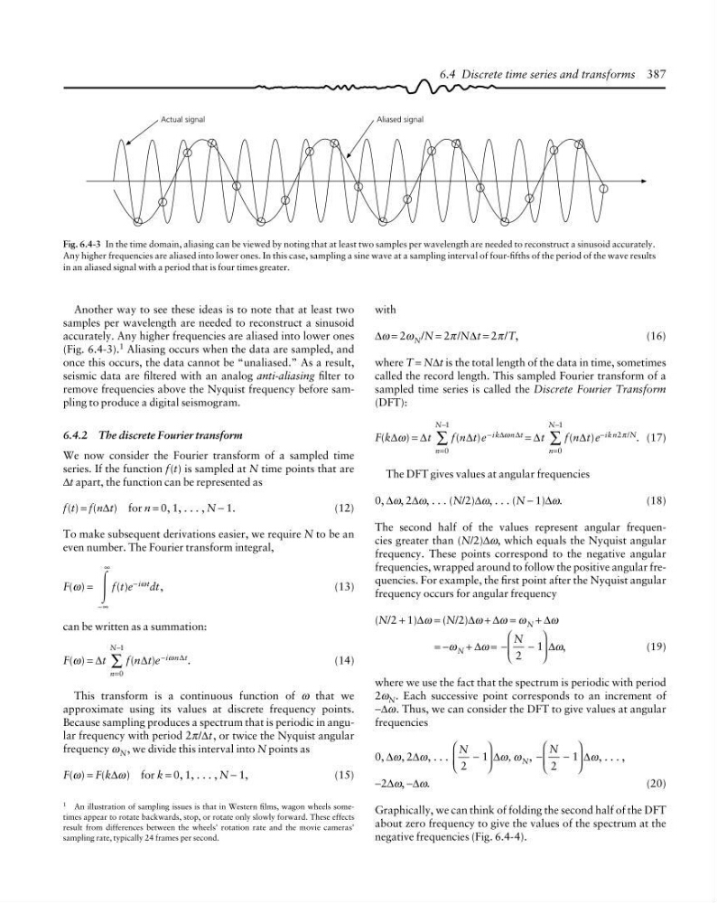
Fig. 6.4-3 In the time domain, aliasing can be viewed by noting that at least two samples per wavelength are needed to reconstruct a sinusoid accurately.
Any higher frequencies are aliased into lower ones. In this case, sampling a sine wave at a sampling interval of four-fifths of the period of the wave results
in an aliased signal with a period that is four times greater.
Another way to see these ideas is to note that at least two
samples per wavelength are needed to reconstruct a sinusoid
accurately. Any higher frequencies are aliased into lower ones
(Fig. 6.4-3). 1 Aliasing occurs when the data are sampled, and
once this occurs, the data cannot be “unaliased.” As a result,
seismic data are filtered with an analog anti-aliasing filter to
remove frequencies above the Nyquist frequency before sampling to produce a digital seismogram.
6.4.2 The discrete Fourier transform
We now consider the Fourier transform of a sampled time
series. If the function f(t) is sampled at N time points that are
∆t apart, the function can be represented as
f(t) = f(n∆t) for n = 0, 1, . . . , N − 1.
(12)
To make subsequent derivations easier, we require N to be an
even number. The Fourier transform integral,
F(ω) =
Ύ
−∞
∞
f(t)e
− iω t
dt,
(13)
can be written as a summation:
F(ω) = ∆t
n
N
=
−
∑
0
1
f(n∆t)e −iω n∆t .
(14)
This transform is a continuous function of ω that we
approximate using its values at discrete frequency points.
Because sampling produces a spectrum that is periodic in angular frequency with period 2π/∆t, or twice the Nyquist angular
frequency ω N , we divide this interval into N points as
F(ω) = F(k∆ω) for k = 0, 1, . . . , N − 1,
(15)
1 An illustration of sampling issues is that in Western films, wagon wheels sometimes appear to rotate backwards, stop, or rotate only slowly forward. These effects
result from differences between the wheels’ rotation rate and the movie cameras’
sampling rate, typically 24 frames per second.
6.4 Discrete time series and transforms 387
with
∆ω = 2ω N /N = 2π /N∆t = 2π /T,
(16)
where T = N∆t is the total length of the data in time, sometimes
called the record length. This sampled Fourier transform of a
sampled time series is called the Discrete Fourier Transform
(DFT):
F(k∆ω) = ∆t
n
N
=
−
∑
0
1
f(n∆t)e − ik∆ω n∆t = ∆t
n
N
=
−
∑
0
1
f(n∆t)e −ikn2π /N . (17)
The DFT gives values at angular frequencies
0, ∆ω, 2∆ω, . . . (N/2)∆ω, . . . (N − 1)∆ω.
(18)
The second half of the values represent angular frequencies greater than (N/2)∆ω, which equals the Nyquist angular
frequency. These points correspond to the negative angular
frequencies, wrapped around to follow the positive angular frequencies. For example, the first point after the Nyquist angular
frequency occurs for angular frequency
(N/2 + 1)∆ω = (N/2)∆ω + ∆ω = ω N + ∆ω
= −ω N + ∆ω = −
−
⎛
⎝
⎜
⎞
⎠
⎟
N
2
1 ∆ω,
(19)
where we use the fact that the spectrum is periodic with period
2ω N . Each successive point corresponds to an increment of
−∆ω. Thus, we can consider the DFT to give values at angular
frequencies
0, ∆ω, 2∆ω, . . .
N
2
1
−
⎛
⎝
⎜
⎞
⎠
⎟ ∆ω, ω N , −
−
⎛
⎝
⎜
⎞
⎠
⎟
N
2
1 ∆ω, . . . ,
−2∆ω, −∆ω.
(20)
Graphically, we can think of folding the second half of the DFT
about zero frequency to give the values of the spectrum at the
negative frequencies (Fig. 6.4-4).
Aliased signal
Fig. 6.4-3 In the time domain, aliasing can be viewed by noting that at least two samples per wavelength are needed to reconstruct a sinusoid accurately.
Any higher frequencies are aliased into lower ones. In this case, sampling a sine wave at a sampling interval of four-fifths of the period of the wave results
in an aliased signal with a period that is four times greater.
Another way to see these ideas is to note that at least two
samples per wavelength are needed to reconstruct a sinusoid
accurately. Any higher frequencies are aliased into lower ones
(Fig. 6.4-3). 1 Aliasing occurs when the data are sampled, and
once this occurs, the data cannot be “unaliased.” As a result,
seismic data are filtered with an analog anti-aliasing filter to
remove frequencies above the Nyquist frequency before sampling to produce a digital seismogram.
6.4.2 The discrete Fourier transform
We now consider the Fourier transform of a sampled time
series. If the function f(t) is sampled at N time points that are
∆t apart, the function can be represented as
f(t) = f(n∆t) for n = 0, 1, . . . , N − 1.
(12)
To make subsequent derivations easier, we require N to be an
even number. The Fourier transform integral,
F(ω) =
Ύ
−∞
∞
f(t)e
− iω t
dt,
(13)
can be written as a summation:
F(ω) = ∆t
n
N
=
−
∑
0
1
f(n∆t)e −iω n∆t .
(14)
This transform is a continuous function of ω that we
approximate using its values at discrete frequency points.
Because sampling produces a spectrum that is periodic in angular frequency with period 2π/∆t, or twice the Nyquist angular
frequency ω N , we divide this interval into N points as
F(ω) = F(k∆ω) for k = 0, 1, . . . , N − 1,
(15)
1 An illustration of sampling issues is that in Western films, wagon wheels sometimes appear to rotate backwards, stop, or rotate only slowly forward. These effects
result from differences between the wheels’ rotation rate and the movie cameras’
sampling rate, typically 24 frames per second.
6.4 Discrete time series and transforms 387
with
∆ω = 2ω N /N = 2π /N∆t = 2π /T,
(16)
where T = N∆t is the total length of the data in time, sometimes
called the record length. This sampled Fourier transform of a
sampled time series is called the Discrete Fourier Transform
(DFT):
F(k∆ω) = ∆t
n
N
=
−
∑
0
1
f(n∆t)e − ik∆ω n∆t = ∆t
n
N
=
−
∑
0
1
f(n∆t)e −ikn2π /N . (17)
The DFT gives values at angular frequencies
0, ∆ω, 2∆ω, . . . (N/2)∆ω, . . . (N − 1)∆ω.
(18)
The second half of the values represent angular frequencies greater than (N/2)∆ω, which equals the Nyquist angular
frequency. These points correspond to the negative angular
frequencies, wrapped around to follow the positive angular frequencies. For example, the first point after the Nyquist angular
frequency occurs for angular frequency
(N/2 + 1)∆ω = (N/2)∆ω + ∆ω = ω N + ∆ω
= −ω N + ∆ω = −
−
⎛
⎝
⎜
⎞
⎠
⎟
N
2
1 ∆ω,
(19)
where we use the fact that the spectrum is periodic with period
2ω N . Each successive point corresponds to an increment of
−∆ω. Thus, we can consider the DFT to give values at angular
frequencies
0, ∆ω, 2∆ω, . . .
N
2
1
−
⎛
⎝
⎜
⎞
⎠
⎟ ∆ω, ω N , −
−
⎛
⎝
⎜
⎞
⎠
⎟
N
2
1 ∆ω, . . . ,
−2∆ω, −∆ω.
(20)
Graphically, we can think of folding the second half of the DFT
about zero frequency to give the values of the spectrum at the
negative frequencies (Fig. 6.4-4).