

388 Seismograms as Signals
Discrete
Fourier
transform
(DFT)
−ω N
0
(N/2)∆
=
ω N
0
ω N
ω
(N − 1)∆ω
Continuous frequency amplitude spectrum
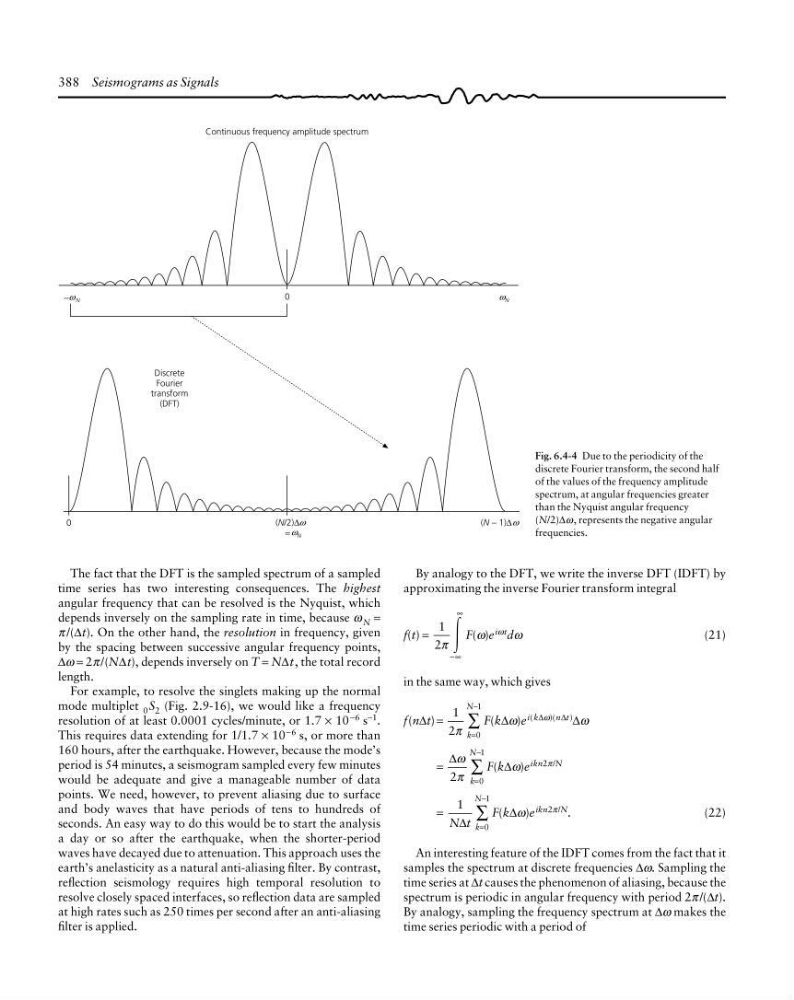
Fig. 6.4-4 Due to the periodicity of the
discrete Fourier transform, the second half
of the values of the frequency amplitude
spectrum, at angular frequencies greater
than the Nyquist angular frequency
(N/2)∆ω, represents the negative angular
frequencies.
The fact that the DFT is the sampled spectrum of a sampled
time series has two interesting consequences. The highest
angular frequency that can be resolved is the Nyquist, which
depends inversely on the sampling rate in time, because ω N =
π /(∆t). On the other hand, the resolution in frequency, given
by the spacing between successive angular frequency points,
∆ω = 2π /(N∆t), depends inversely on T = N∆t, the total record
length.
For example, to resolve the singlets making up the normal
mode multiplet 0 S 2 (Fig. 2.9-16), we would like a frequency
resolution of at least 0.0001 cycles/minute, or 1.7 × 10 −6 s −1 .
This requires data extending for 1/1.7 × 10 −6 s, or more than
160 hours, after the earthquake. However, because the mode’s
period is 54 minutes, a seismogram sampled every few minutes
would be adequate and give a manageable number of data
points. We need, however, to prevent aliasing due to surface
and body waves that have periods of tens to hundreds of
seconds. An easy way to do this would be to start the analysis
a day or so after the earthquake, when the shorter-period
waves have decayed due to attenuation. This approach uses the
earth’s anelasticity as a natural anti-aliasing filter. By contrast,
reflection seismology requires high temporal resolution to
resolve closely spaced interfaces, so reflection data are sampled
at high rates such as 250 times per second after an anti-aliasing
filter is applied.
By analogy to the DFT, we write the inverse DFT (IDFT) by
approximating the inverse Fourier transform integral
f(t) =
1
2π Ύ
−∞
∞
F(ω)e iωt dω
(21)
in the same way, which gives
f(n∆t) =
1
2π k
N
=
−
∑
0
1
F(k∆ω)e i(k∆ω)(n∆t) ∆ω
=
∆ω
π
2 k
N
=
−
∑
0
1
F(k∆ω)e ikn2π/N
=
1
N t
∆ k
N
=
−
∑
0
1
F(k∆ω)e ikn2π/N .
(22)
An interesting feature of the IDFT comes from the fact that it
samples the spectrum at discrete frequencies ∆ω. Sampling the
time series at ∆t causes the phenomenon of aliasing, because the
spectrum is periodic in angular frequency with period 2π /(∆t).
By analogy, sampling the frequency spectrum at ∆ω makes the
time series periodic with a period of
Discrete
Fourier
transform
(DFT)
−ω N
0
(N/2)∆
=
ω N
0
ω N
ω
(N − 1)∆ω
Continuous frequency amplitude spectrum
Fig. 6.4-4 Due to the periodicity of the
discrete Fourier transform, the second half
of the values of the frequency amplitude
spectrum, at angular frequencies greater
than the Nyquist angular frequency
(N/2)∆ω, represents the negative angular
frequencies.
The fact that the DFT is the sampled spectrum of a sampled
time series has two interesting consequences. The highest
angular frequency that can be resolved is the Nyquist, which
depends inversely on the sampling rate in time, because ω N =
π /(∆t). On the other hand, the resolution in frequency, given
by the spacing between successive angular frequency points,
∆ω = 2π /(N∆t), depends inversely on T = N∆t, the total record
length.
For example, to resolve the singlets making up the normal
mode multiplet 0 S 2 (Fig. 2.9-16), we would like a frequency
resolution of at least 0.0001 cycles/minute, or 1.7 × 10 −6 s −1 .
This requires data extending for 1/1.7 × 10 −6 s, or more than
160 hours, after the earthquake. However, because the mode’s
period is 54 minutes, a seismogram sampled every few minutes
would be adequate and give a manageable number of data
points. We need, however, to prevent aliasing due to surface
and body waves that have periods of tens to hundreds of
seconds. An easy way to do this would be to start the analysis
a day or so after the earthquake, when the shorter-period
waves have decayed due to attenuation. This approach uses the
earth’s anelasticity as a natural anti-aliasing filter. By contrast,
reflection seismology requires high temporal resolution to
resolve closely spaced interfaces, so reflection data are sampled
at high rates such as 250 times per second after an anti-aliasing
filter is applied.
By analogy to the DFT, we write the inverse DFT (IDFT) by
approximating the inverse Fourier transform integral
f(t) =
1
2π Ύ
−∞
∞
F(ω)e iωt dω
(21)
in the same way, which gives
f(n∆t) =
1
2π k
N
=
−
∑
0
1
F(k∆ω)e i(k∆ω)(n∆t) ∆ω
=
∆ω
π
2 k
N
=
−
∑
0
1
F(k∆ω)e ikn2π/N
=
1
N t
∆ k
N
=
−
∑
0
1
F(k∆ω)e ikn2π/N .
(22)
An interesting feature of the IDFT comes from the fact that it
samples the spectrum at discrete frequencies ∆ω. Sampling the
time series at ∆t causes the phenomenon of aliasing, because the
spectrum is periodic in angular frequency with period 2π /(∆t).
By analogy, sampling the frequency spectrum at ∆ω makes the
time series periodic with a period of