

Fig. 6.3-13 Illustration showing that a function has the same
auto-correlation if it is reversed in time.
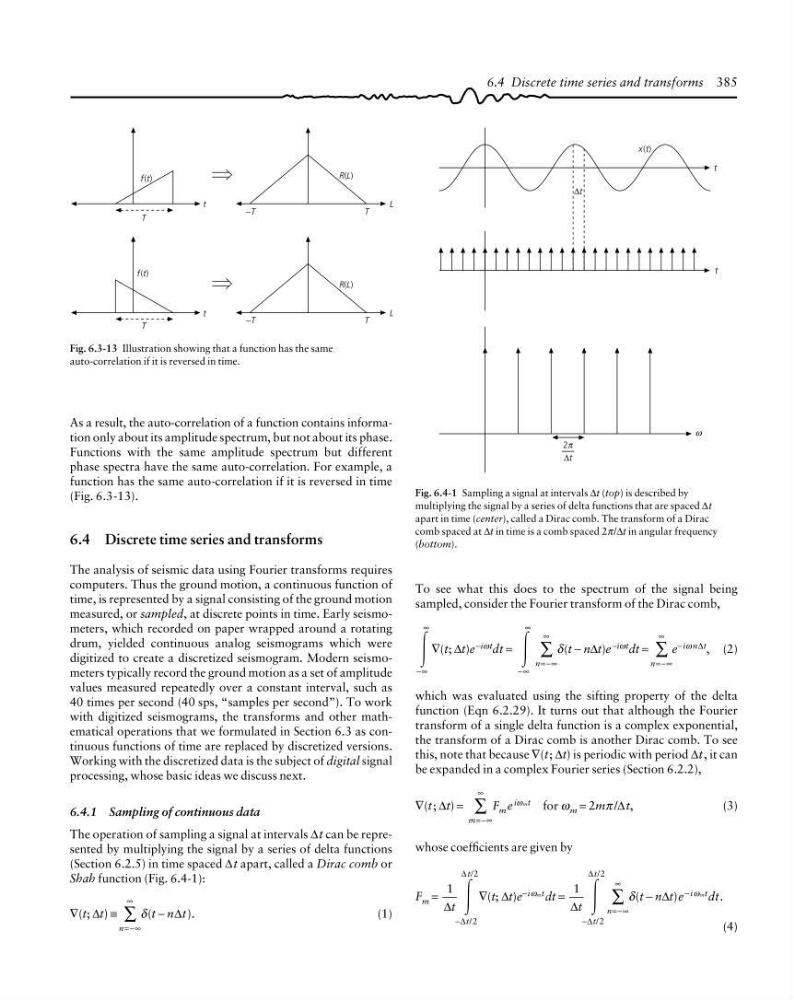
Fig. 6.4-1 Sampling a signal at intervals ∆t (top) is described by
multiplying the signal by a series of delta functions that are spaced ∆t
apart in time (center), called a Dirac comb. The transform of a Dirac
comb spaced at ∆t in time is a comb spaced 2π/∆t in angular frequency
(bottom).
f(t)
R(L)
−T
T
−T
T
t
T
R(L)
t
f(t)
T
L
L
As a result, the auto-correlation of a function contains information only about its amplitude spectrum, but not about its phase.
Functions with the same amplitude spectrum but different
phase spectra have the same auto-correlation. For example, a
function has the same auto-correlation if it is reversed in time
(Fig. 6.3-13).
6.4 Discrete time series and transforms
The analysis of seismic data using Fourier transforms requires
computers. Thus the ground motion, a continuous function of
time, is represented by a signal consisting of the ground motion
measured, or sampled, at discrete points in time. Early seismometers, which recorded on paper wrapped around a rotating
drum, yielded continuous analog seismograms which were
digitized to create a discretized seismogram. Modern seismometers typically record the ground motion as a set of amplitude
values measured repeatedly over a constant interval, such as
40 times per second (40 sps, “samples per second”). To work
with digitized seismograms, the transforms and other mathematical operations that we formulated in Section 6.3 as continuous functions of time are replaced by discretized versions.
Working with the discretized data is the subject of digital signal
processing, whose basic ideas we discuss next.
6.4.1 Sampling of continuous data
The operation of sampling a signal at intervals ∆t can be represented by multiplying the signal by a series of delta functions
(Section 6.2.5) in time spaced ∆t apart, called a Dirac comb or
Shah function (Fig. 6.4-1):
∇(t; ∆t) ≡
n=−∞
∞
∑ δ(t − n∆t).
(1)
To see what this does to the spectrum of the signal being
sampled, consider the Fourier transform of the Dirac comb,
Ύ
−∞
∞
∇(t; ∆t)e −iωt dt =
Ύ
−∞
∞
n=−∞
∞
∑ δ(t − n∆t)e −iωt dt =
n=−∞
∞
∑ e −iω n∆t , (2)
which was evaluated using the sifting property of the delta
function (Eqn 6.2.29). It turns out that although the Fourier
transform of a single delta function is a complex exponential,
the transform of a Dirac comb is another Dirac comb. To see
this, note that because ∇(t; ∆t) is periodic with period ∆t, it can
be expanded in a complex Fourier series (Section 6.2.2),
∇(t; ∆t) =
m=−∞
∞
∑ F m e iωmt for ω m = 2mπ /∆t,
(3)
whose coefficients are given by
F m =
1
2
2
∆
∆
∆
t
t
t
Ύ
− /
/
∇(t; ∆t)e −iωmt dt =
1
2
2
∆
∆
∆
t
t
t
Ύ
− /
/
n=−∞
∞
∑ δ(t − n∆t)e − iωmt dt.
(4)
6.4 Discrete time series and transforms 385
2π
∆t
∆t
x(t)
t
t
π
ω
auto-correlation if it is reversed in time.
Fig. 6.4-1 Sampling a signal at intervals ∆t (top) is described by
multiplying the signal by a series of delta functions that are spaced ∆t
apart in time (center), called a Dirac comb. The transform of a Dirac
comb spaced at ∆t in time is a comb spaced 2π/∆t in angular frequency
(bottom).
f(t)
R(L)
−T
T
−T
T
t
T
R(L)
t
f(t)
T
L
L
As a result, the auto-correlation of a function contains information only about its amplitude spectrum, but not about its phase.
Functions with the same amplitude spectrum but different
phase spectra have the same auto-correlation. For example, a
function has the same auto-correlation if it is reversed in time
(Fig. 6.3-13).
6.4 Discrete time series and transforms
The analysis of seismic data using Fourier transforms requires
computers. Thus the ground motion, a continuous function of
time, is represented by a signal consisting of the ground motion
measured, or sampled, at discrete points in time. Early seismometers, which recorded on paper wrapped around a rotating
drum, yielded continuous analog seismograms which were
digitized to create a discretized seismogram. Modern seismometers typically record the ground motion as a set of amplitude
values measured repeatedly over a constant interval, such as
40 times per second (40 sps, “samples per second”). To work
with digitized seismograms, the transforms and other mathematical operations that we formulated in Section 6.3 as continuous functions of time are replaced by discretized versions.
Working with the discretized data is the subject of digital signal
processing, whose basic ideas we discuss next.
6.4.1 Sampling of continuous data
The operation of sampling a signal at intervals ∆t can be represented by multiplying the signal by a series of delta functions
(Section 6.2.5) in time spaced ∆t apart, called a Dirac comb or
Shah function (Fig. 6.4-1):
∇(t; ∆t) ≡
n=−∞
∞
∑ δ(t − n∆t).
(1)
To see what this does to the spectrum of the signal being
sampled, consider the Fourier transform of the Dirac comb,
Ύ
−∞
∞
∇(t; ∆t)e −iωt dt =
Ύ
−∞
∞
n=−∞
∞
∑ δ(t − n∆t)e −iωt dt =
n=−∞
∞
∑ e −iω n∆t , (2)
which was evaluated using the sifting property of the delta
function (Eqn 6.2.29). It turns out that although the Fourier
transform of a single delta function is a complex exponential,
the transform of a Dirac comb is another Dirac comb. To see
this, note that because ∇(t; ∆t) is periodic with period ∆t, it can
be expanded in a complex Fourier series (Section 6.2.2),
∇(t; ∆t) =
m=−∞
∞
∑ F m e iωmt for ω m = 2mπ /∆t,
(3)
whose coefficients are given by
F m =
1
2
2
∆
∆
∆
t
t
t
Ύ
− /
/
∇(t; ∆t)e −iωmt dt =
1
2
2
∆
∆
∆
t
t
t
Ύ
− /
/
n=−∞
∞
∑ δ(t − n∆t)e − iωmt dt.
(4)
6.4 Discrete time series and transforms 385
2π
∆t
∆t
x(t)
t
t
π
ω