

384 Seismograms as Signals
Fig. 6.3-12 Illustration, for a boxcar function, that the auto-correlation is
maximum at zero lag and is an even function of the lag.
The auto-correlation is significant in the theory of filtering
because it is related to the amplitude spectrum. To see this,
consider a function f(t) that is zero except between −T/2 and
T/2. The auto-correlation
R L
T
f t f t L dt
T
T
T
( ) lim
( ) (
)
/
/
=
+
→∞
−
1
2
2
Ύ
(28)
can be expanded using the inverse Fourier transform and using
the time shift theorem (Section 6.2.4),
R L
T
f t
F e
d dt
T
T
T
i t L
( ) lim
( )
( )
/
/
(
)
=
⎡
⎣
⎢
⎢
⎢
⎤
⎦
⎥
⎥
⎥
→∞
−
−∞
∞
+
1
2
2
2
π
ω
ω
ω
Ύ Ύ
=
⎡
⎣
⎢
⎢
⎢
⎤
⎦
⎥
⎥
⎥
→∞
−∞
∞
−
lim
( )
( )
/
/
T
i L
T
T
i t
T
F e
f t e dt d
1
2
2
2
π
ω
ω
ω
ω
Ύ
Ύ
=
−
→∞
−∞
∞
lim
( ) ( )
T
i L
T
F F
e d
1
2π
ω
ω
ω
ω
Ύ
=
→∞
−∞
∞
lim
( )
,
T
i L
T
F
e d
1
2
2
π
ω
ω
ω
Ύ
|
|
(29)
where the last step uses the fact that F (−ω) = F*(ω). Thus, if
we define the power spectrum, a normalized version of the
amplitude spectrum,
P(ω) = lim
T
T
→∞
1 | F(ω) | 2 ,
(30)
we see that the auto-correlation is the inverse Fourier transform
of the power spectrum:
R(L) =
1
2π Ύ
−∞
∞
| P(ω) |e iωL dω.
(31)
f(t)
T
R(L)
L
T
−T
t
R L
T
f t f t L dt
T
T
T
( ) lim
( ) (
) .
/
/
=
+
→∞
−
1
2
2
Ύ
(27)
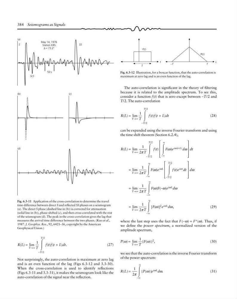
Not surprisingly, the auto-correlation is maximum at zero lag
and is an even function of the lag (Figs 6.3-12 and 3.3-30).
When the cross-correlation is used to identify reflections
(Figs 6.3-11 and 3.3-31), it makes the seismogram look like the
auto-correlation of the signal near the reflection.
(a)
(b)
(d)
(c)
S
May 14, 1976
Station KBS
∆ = 73.2°
SS
ScS
50 s
Fig. 6.3-11 Application of the cross-correlation to determine the travel
time difference between direct S and reflected SS phases on a seismogram
(a). The direct S phase (dashed line in (b)) is corrected for attenuation
(solid line in (b)), phase-shifted (c), and then cross-correlated with the rest
of the seismogram (d). The peak in the cross-correlation gives the lag that
measures the arrival time difference between the two phases. (Kuo et al.,
1987. J. Geophys. Res., 92, 6421–36, copyright by the American
Geophysical Union.)
Fig. 6.3-12 Illustration, for a boxcar function, that the auto-correlation is
maximum at zero lag and is an even function of the lag.
The auto-correlation is significant in the theory of filtering
because it is related to the amplitude spectrum. To see this,
consider a function f(t) that is zero except between −T/2 and
T/2. The auto-correlation
R L
T
f t f t L dt
T
T
T
( ) lim
( ) (
)
/
/
=
+
→∞
−
1
2
2
Ύ
(28)
can be expanded using the inverse Fourier transform and using
the time shift theorem (Section 6.2.4),
R L
T
f t
F e
d dt
T
T
T
i t L
( ) lim
( )
( )
/
/
(
)
=
⎡
⎣
⎢
⎢
⎢
⎤
⎦
⎥
⎥
⎥
→∞
−
−∞
∞
+
1
2
2
2
π
ω
ω
ω
Ύ Ύ
=
⎡
⎣
⎢
⎢
⎢
⎤
⎦
⎥
⎥
⎥
→∞
−∞
∞
−
lim
( )
( )
/
/
T
i L
T
T
i t
T
F e
f t e dt d
1
2
2
2
π
ω
ω
ω
ω
Ύ
Ύ
=
−
→∞
−∞
∞
lim
( ) ( )
T
i L
T
F F
e d
1
2π
ω
ω
ω
ω
Ύ
=
→∞
−∞
∞
lim
( )
,
T
i L
T
F
e d
1
2
2
π
ω
ω
ω
Ύ
|
|
(29)
where the last step uses the fact that F (−ω) = F*(ω). Thus, if
we define the power spectrum, a normalized version of the
amplitude spectrum,
P(ω) = lim
T
T
→∞
1 | F(ω) | 2 ,
(30)
we see that the auto-correlation is the inverse Fourier transform
of the power spectrum:
R(L) =
1
2π Ύ
−∞
∞
| P(ω) |e iωL dω.
(31)
f(t)
T
R(L)
L
T
−T
t
R L
T
f t f t L dt
T
T
T
( ) lim
( ) (
) .
/
/
=
+
→∞
−
1
2
2
Ύ
(27)
Not surprisingly, the auto-correlation is maximum at zero lag
and is an even function of the lag (Figs 6.3-12 and 3.3-30).
When the cross-correlation is used to identify reflections
(Figs 6.3-11 and 3.3-31), it makes the seismogram look like the
auto-correlation of the signal near the reflection.
(a)
(b)
(d)
(c)
S
May 14, 1976
Station KBS
∆ = 73.2°
SS
ScS
50 s
Fig. 6.3-11 Application of the cross-correlation to determine the travel
time difference between direct S and reflected SS phases on a seismogram
(a). The direct S phase (dashed line in (b)) is corrected for attenuation
(solid line in (b)), phase-shifted (c), and then cross-correlated with the rest
of the seismogram (d). The peak in the cross-correlation gives the lag that
measures the arrival time difference between the two phases. (Kuo et al.,
1987. J. Geophys. Res., 92, 6421–36, copyright by the American
Geophysical Union.)