

similar to that of finite record length. Longer records broaden
the peaks less, and so give better estimates of attenuation up to
the point where the effects of noise degrade the estimates.
Though we can never get around the problem of finite record
length, it can be ameliorated by using a different window function than a boxcar. A window function whose “corners” are
less “sharp,” known as a taper, reduces the size of the side lobes
and thus the distortion. One simple such function, a cosine
taper, is a boxcar with smoother ends:
W t
t T T
T
( )
cos
(
)
=
+
+ −
⎡
⎣
⎢
⎢
⎤
⎦
⎥
⎥
1
2
1
1
1
π
for −T < t < −T + T 1
= 1
for −T + T 1 ≤ t ≤ T − T 1
=
+
− +
⎡
⎣
⎢
⎢
⎤
⎦
⎥
⎥
cos
(
)
1
2
1
1
1
π t T T
T
for T − T 1 < t < T
= 0
for other times.
(25)
The parameter T 1 is the tapered fraction of the half-length T.
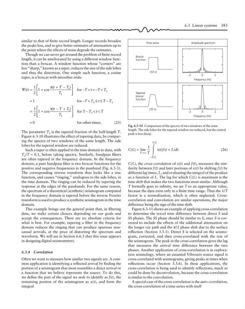
Figure 6.3-10 illustrates the effect of tapering data, by comparing the spectra of two windows of the same length. The side
lobes for the tapered window are reduced.
Such a taper is often applied in the time domain to data, with
T 1 /T ≈ 0.1, before taking spectra. Similarly, bandpass filters
are often tapered in the frequency domain. In the frequency
domain, a pure bandpass filter is two boxcar functions for the
positive and negative frequencies in the passband (Fig. 6.3-3).
The corresponding inverse transform thus looks like a sinc
function, and causes “ringing,” analogous to the side lobes, in
the time domain. The ringing can be reduced by tapering the
response at the edges of the passbands. For the same reason,
the spectrum of a theoretical (synthetic) seismogram computed
in the frequency domain is tapered before the inverse Fourier
transform is used to produce a synthetic seismogram in the time
domain.
This example brings out the general point that, in filtering
data, we make certain choices depending on our goals and
accept the consequences. There are no absolute criteria for
what is best. For example, tapering a filter in the frequency
domain reduces the ringing that can produce spurious noncausal arrivals, at the price of distorting the spectrum and
waveform. We will see in Section 6.6.5 that this issue appears
in designing digital seismometers.
6.3.4 Correlation
Often we want to measure how similar two signals are. A common application is identifying a reflected arrival by finding the
portion of a seismogram that most resembles a direct arrival or
a function that we believe represents the source. To do this,
we define the part of the signal we seek to identify as f(t), the
remaining portion of the seismogram as x(t), and form the
integral
C L
T
x t f t L dt
T
T
T
( ) lim
( ) (
) .
/
/
=
+
→∞
−
1
2
2
Ύ
(26)
C(L), the cross-correlation of x(t) and f(t), measures the similarity between f(t) and later portions of x(t) by shifting f(t) by
different lag times, L, and evaluating the integral of the product
as a function of L. The lag for which C(L) is maximum is the
time shift that makes the two functions most similar. Although
T formally goes to infinity, we set T to an appropriate value,
because the data exist only in a finite time range. Thus the 1/T
factor is a normalization, which is often neglected. Crosscorrelation and convolution are similar operations, the major
difference being the sign of the time shift.
Figure 6.3-11 shows an example of applying cross-correlation
to determine the travel time difference between direct S and
SS phases. The SS phase should be similar to S, once S is corrected to include the effects of the additional attenuation on
the longer ray path and the π /2 phase shift due to the surface
reflection (Section 3.5.1). Direct S is selected on the seismogram, corrected, and then cross-correlated with the rest of
the seismogram. The peak in the cross-correlation gives the lag
that measures the arrival time difference between the two
phases. Another application of cross-correlation is in exploration seismology, where an assumed Vibroseis source signal is
cross-correlated with seismograms, giving peaks at times when
reflections occur (Section 3.3.6). In these applications, the
cross-correlation is being used to identify reflections, much as
could be done by deconvolution, because the cross-correlation
is similar to the convolution.
A special case of the cross-correlation is the auto-correlation,
the cross-correlation of a time series with itself
6.3 Linear systems 383
Boxcar
function
| 32 s |
| 32 s |
Tapered
boxcar
function
−2
2
0
Frequency (Hz)
−2
2
0
Frequency (Hz)
Time series
Amplitude spectrum
Fig. 6.3-10 Comparison of the spectra of two windows of the same
length. The side lobes for the tapered window are reduced, but the central
peak is less sharp.
the peaks less, and so give better estimates of attenuation up to
the point where the effects of noise degrade the estimates.
Though we can never get around the problem of finite record
length, it can be ameliorated by using a different window function than a boxcar. A window function whose “corners” are
less “sharp,” known as a taper, reduces the size of the side lobes
and thus the distortion. One simple such function, a cosine
taper, is a boxcar with smoother ends:
W t
t T T
T
( )
cos
(
)
=
+
+ −
⎡
⎣
⎢
⎢
⎤
⎦
⎥
⎥
1
2
1
1
1
π
for −T < t < −T + T 1
= 1
for −T + T 1 ≤ t ≤ T − T 1
=
+
− +
⎡
⎣
⎢
⎢
⎤
⎦
⎥
⎥
cos
(
)
1
2
1
1
1
π t T T
T
for T − T 1 < t < T
= 0
for other times.
(25)
The parameter T 1 is the tapered fraction of the half-length T.
Figure 6.3-10 illustrates the effect of tapering data, by comparing the spectra of two windows of the same length. The side
lobes for the tapered window are reduced.
Such a taper is often applied in the time domain to data, with
T 1 /T ≈ 0.1, before taking spectra. Similarly, bandpass filters
are often tapered in the frequency domain. In the frequency
domain, a pure bandpass filter is two boxcar functions for the
positive and negative frequencies in the passband (Fig. 6.3-3).
The corresponding inverse transform thus looks like a sinc
function, and causes “ringing,” analogous to the side lobes, in
the time domain. The ringing can be reduced by tapering the
response at the edges of the passbands. For the same reason,
the spectrum of a theoretical (synthetic) seismogram computed
in the frequency domain is tapered before the inverse Fourier
transform is used to produce a synthetic seismogram in the time
domain.
This example brings out the general point that, in filtering
data, we make certain choices depending on our goals and
accept the consequences. There are no absolute criteria for
what is best. For example, tapering a filter in the frequency
domain reduces the ringing that can produce spurious noncausal arrivals, at the price of distorting the spectrum and
waveform. We will see in Section 6.6.5 that this issue appears
in designing digital seismometers.
6.3.4 Correlation
Often we want to measure how similar two signals are. A common application is identifying a reflected arrival by finding the
portion of a seismogram that most resembles a direct arrival or
a function that we believe represents the source. To do this,
we define the part of the signal we seek to identify as f(t), the
remaining portion of the seismogram as x(t), and form the
integral
C L
T
x t f t L dt
T
T
T
( ) lim
( ) (
) .
/
/
=
+
→∞
−
1
2
2
Ύ
(26)
C(L), the cross-correlation of x(t) and f(t), measures the similarity between f(t) and later portions of x(t) by shifting f(t) by
different lag times, L, and evaluating the integral of the product
as a function of L. The lag for which C(L) is maximum is the
time shift that makes the two functions most similar. Although
T formally goes to infinity, we set T to an appropriate value,
because the data exist only in a finite time range. Thus the 1/T
factor is a normalization, which is often neglected. Crosscorrelation and convolution are similar operations, the major
difference being the sign of the time shift.
Figure 6.3-11 shows an example of applying cross-correlation
to determine the travel time difference between direct S and
SS phases. The SS phase should be similar to S, once S is corrected to include the effects of the additional attenuation on
the longer ray path and the π /2 phase shift due to the surface
reflection (Section 3.5.1). Direct S is selected on the seismogram, corrected, and then cross-correlated with the rest of
the seismogram. The peak in the cross-correlation gives the lag
that measures the arrival time difference between the two
phases. Another application of cross-correlation is in exploration seismology, where an assumed Vibroseis source signal is
cross-correlated with seismograms, giving peaks at times when
reflections occur (Section 3.3.6). In these applications, the
cross-correlation is being used to identify reflections, much as
could be done by deconvolution, because the cross-correlation
is similar to the convolution.
A special case of the cross-correlation is the auto-correlation,
the cross-correlation of a time series with itself
6.3 Linear systems 383
Boxcar
function
| 32 s |
| 32 s |
Tapered
boxcar
function
−2
2
0
Frequency (Hz)
−2
2
0
Frequency (Hz)
Time series
Amplitude spectrum
Fig. 6.3-10 Comparison of the spectra of two windows of the same
length. The side lobes for the tapered window are reduced, but the central
peak is less sharp.