

382 Seismograms as Signals
Amplitude spectrum
–2
0
2
Frequency (Hz)
Sine function with
period of 10 s
| 20 s |
–2
0
2
Frequency (Hz)
–2
0
2
Frequency (Hz)
–2
0
2
Frequency (Hz)
–2
0
2
Frequency (Hz)
(a)
(a) sampled
for a total of 48 s
| 20 s |
(b)
Sum of 2 sine
functions with 10 s and 20 s periods
| 20 s |
(c)
(c) sampled
for a total of 36 s
| 20 s |
(d)
(c) sampled
for a total of 24 s
| 20 s |
(e)
Time series
Data length and frequency resolution
two peaks can be resolved, is proportional to the reciprocal of
the record length.
This relation between signals in the time and frequency
domains demonstrates a fundamental principle. By taking a
finite length portion of a time function, we broaden and distort
its spectrum in a predictable way. The reverse occurs in the frequency domain; taking a finite portion of the spectrum distorts
the time function, as we discussed in considering Fig. 6.3-3.
For example, because a seismometer only responds to ground
motion in a certain frequency range, the resulting seismogram
is a somewhat distorted record of the ground motion. Similarly, physical processes like anelasticity (Section 3.7.8) and
diffraction (Section 2.5.10) that remove high frequencies distort the resulting waveforms.
Thus we have an “uncertainty principle” that the product of
the “widths” in the two domains is constant; for a time domain
record with duration T, the resolution in the frequency domain
is proportional to 1/T. Perfect resolution in frequency requires
infinite record length in time, and infinite bandwidth in frequency is needed to represent a time function exactly. These
properties are general features of Fourier transform pairs, so
also apply to distance and wavenumber. 3
The sinc or | sin x/x | function, which we used to represent
taking a finite portion of a time series, appears in other similar
applications. We saw that diffraction through a slit, in which
only part of a wave front is transmitted, is described by a sinc
function (Fig. 2.5-18). The sinc function also describes the
spectrum of waves radiated from a finite fault (Section 4.6.2).
In real cases, we do not have infinite lengths of data. Moreover, it is not always desirable to take more data. For example,
the signal of interest on a seismogram eventually decays into
the noise due to attenuation, or is interferred with by a different
signal. We seek the best resolution of the spectrum of the signal
of interest, but as the record length increases, the noise has a
greater effect and increasingly contaminates the spectrum. We
thus select a compromise record length and try to obtain the
best spectrum. This issue arises in estimating seismic attenuation, which broadens spectral peaks (Section 3.7.7) in a way
Amplitude spectrum: B(ω)
Time series: b(t)
−6π
T
−4π
T
−2π
T
2π
T
4π
T
6π
T
0
Time (t)
Frequency (ω)
−T
T
0
ω
ω
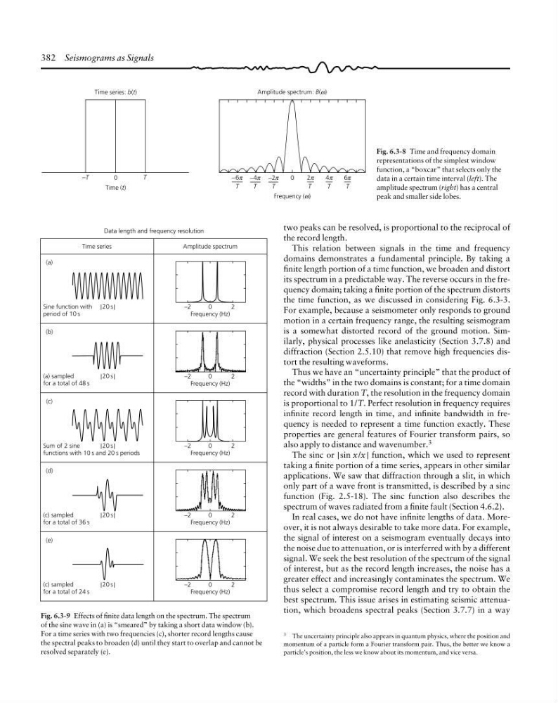
Fig. 6.3-8 Time and frequency domain
representations of the simplest window
function, a “boxcar” that selects only the
data in a certain time interval (left). The
amplitude spectrum (right) has a central
peak and smaller side lobes.
3 The uncertainty principle also appears in quantum physics, where the position and
momentum of a particle form a Fourier transform pair. Thus, the better we know a
particle’s position, the less we know about its momentum, and vice versa.
Fig. 6.3-9 Effects of finite data length on the spectrum. The spectrum
of the sine wave in (a) is “smeared” by taking a short data window (b).
For a time series with two frequencies (c), shorter record lengths cause
the spectral peaks to broaden (d) until they start to overlap and cannot be
resolved separately (e).
Amplitude spectrum
–2
0
2
Frequency (Hz)
Sine function with
period of 10 s
| 20 s |
–2
0
2
Frequency (Hz)
–2
0
2
Frequency (Hz)
–2
0
2
Frequency (Hz)
–2
0
2
Frequency (Hz)
(a)
(a) sampled
for a total of 48 s
| 20 s |
(b)
Sum of 2 sine
functions with 10 s and 20 s periods
| 20 s |
(c)
(c) sampled
for a total of 36 s
| 20 s |
(d)
(c) sampled
for a total of 24 s
| 20 s |
(e)
Time series
Data length and frequency resolution
two peaks can be resolved, is proportional to the reciprocal of
the record length.
This relation between signals in the time and frequency
domains demonstrates a fundamental principle. By taking a
finite length portion of a time function, we broaden and distort
its spectrum in a predictable way. The reverse occurs in the frequency domain; taking a finite portion of the spectrum distorts
the time function, as we discussed in considering Fig. 6.3-3.
For example, because a seismometer only responds to ground
motion in a certain frequency range, the resulting seismogram
is a somewhat distorted record of the ground motion. Similarly, physical processes like anelasticity (Section 3.7.8) and
diffraction (Section 2.5.10) that remove high frequencies distort the resulting waveforms.
Thus we have an “uncertainty principle” that the product of
the “widths” in the two domains is constant; for a time domain
record with duration T, the resolution in the frequency domain
is proportional to 1/T. Perfect resolution in frequency requires
infinite record length in time, and infinite bandwidth in frequency is needed to represent a time function exactly. These
properties are general features of Fourier transform pairs, so
also apply to distance and wavenumber. 3
The sinc or | sin x/x | function, which we used to represent
taking a finite portion of a time series, appears in other similar
applications. We saw that diffraction through a slit, in which
only part of a wave front is transmitted, is described by a sinc
function (Fig. 2.5-18). The sinc function also describes the
spectrum of waves radiated from a finite fault (Section 4.6.2).
In real cases, we do not have infinite lengths of data. Moreover, it is not always desirable to take more data. For example,
the signal of interest on a seismogram eventually decays into
the noise due to attenuation, or is interferred with by a different
signal. We seek the best resolution of the spectrum of the signal
of interest, but as the record length increases, the noise has a
greater effect and increasingly contaminates the spectrum. We
thus select a compromise record length and try to obtain the
best spectrum. This issue arises in estimating seismic attenuation, which broadens spectral peaks (Section 3.7.7) in a way
Amplitude spectrum: B(ω)
Time series: b(t)
−6π
T
−4π
T
−2π
T
2π
T
4π
T
6π
T
0
Time (t)
Frequency (ω)
−T
T
0
ω
ω
Fig. 6.3-8 Time and frequency domain
representations of the simplest window
function, a “boxcar” that selects only the
data in a certain time interval (left). The
amplitude spectrum (right) has a central
peak and smaller side lobes.
3 The uncertainty principle also appears in quantum physics, where the position and
momentum of a particle form a Fourier transform pair. Thus, the better we know a
particle’s position, the less we know about its momentum, and vice versa.
Fig. 6.3-9 Effects of finite data length on the spectrum. The spectrum
of the sine wave in (a) is “smeared” by taking a short data window (b).
For a time series with two frequencies (c), shorter record lengths cause
the spectral peaks to broaden (d) until they start to overlap and cannot be
resolved separately (e).