

Converted phase ray diagram
P p
P m
p
P p
P m
s
P p
S m
s
P s
S m
s
P p
P s
S wave
3-component
seismic station
Moho
p la n e P w a v e
P wave
In c id e n t
Direct
P
P s
conversion
Synthetic radial receiver function
P p P m s
P p S m s
+
P s P m s
P s S m s
5 s
G
B
F
d
d
( )
( )
( ) (
)
,
ω
π
ω
ω δω ω ω ω
ω
=
−
−
⎡
⎣
⎢
⎢
⎢
⎤
⎦
⎥
⎥
⎥
−∞
∞
−∞
∞
1
2 Ύ Ύ
′
″
′
″
″
′
(21)
and using the sifting property (Eqn 6.2.29) to obtain
G(ω) =
1
2π Ύ
−∞
∞
B(ω ′)F(ω − ω′)dω ′ =
1
2π
B(ω) * F(ω).
(22)
Thus the effect of multiplying a time series by a window function is that the spectrum of the time series is convolved with the
spectrum of the window function. This is an example of the
fact that just as convolution in the time domain corresponds
to multiplication in the frequency domain, so multiplication in
the time domain corresponds to convolution in the frequency
domain.
To see the effect of windowing on the spectrum, consider the
simplest window function, a “boxcar” which describes taking
only the data in a certain time interval (Fig. 6.3-8),
b(t) = 1 for −T < t < T,
= 0 otherwise.
(23)
Its Fourier transform is
B
e
d t
e
i
T
T
T
T
T
T
i t
i t
T
T
( )
sin
sin
,
ω
ω
ω
ω
ω
ω
ω
ω
=
=−
=
=
−
−
−
−
Ύ
2
2
(24)
whose amplitude spectrum |B(ω) | has a characteristic shape
with a central lobe and smaller side lobes, and equals zero
where x = ωT = 2nπ. The width of the central lobe is 2π /T.
This | (sin x)/x | curve, sometimes called a sinc function, is
convolved with, and thus modifies, the spectrum |F(ω) |.
For example, if f(t) is a sine wave (Fig. 6.3-9a) whose amplitude spectrum is described by two delta functions, convolution
with B(ω) yields the spectrum of a finite length sine wave, two
sinc functions. Thus, taking a finite length of record “smears”
the delta functions of the infinite length record’s spectrum into
broader peaks with side lobes (Figs 6.3-9b). Taking longer
records (increasing T ) yields sharper spectra (more like the
delta function), because the width of the central lobe of the sinc
function is proportional to 1/T.
This effect has an important consequence for analyzing
signals containing different frequencies, as shown in Fig. 6.3-9c
for a time series with two frequencies. For shorter record
lengths (Figs 6.3-9d and e), the spectral peaks broaden until
they start to overlap and cannot be resolved separately. Once
the width in frequency of the central lobe of the sinc function exceeds the separation between the two spectral peaks
(Figs 6.3-9e), they cannot be resolved. Thus the frequency
resolution, the minimum separation in frequency for which
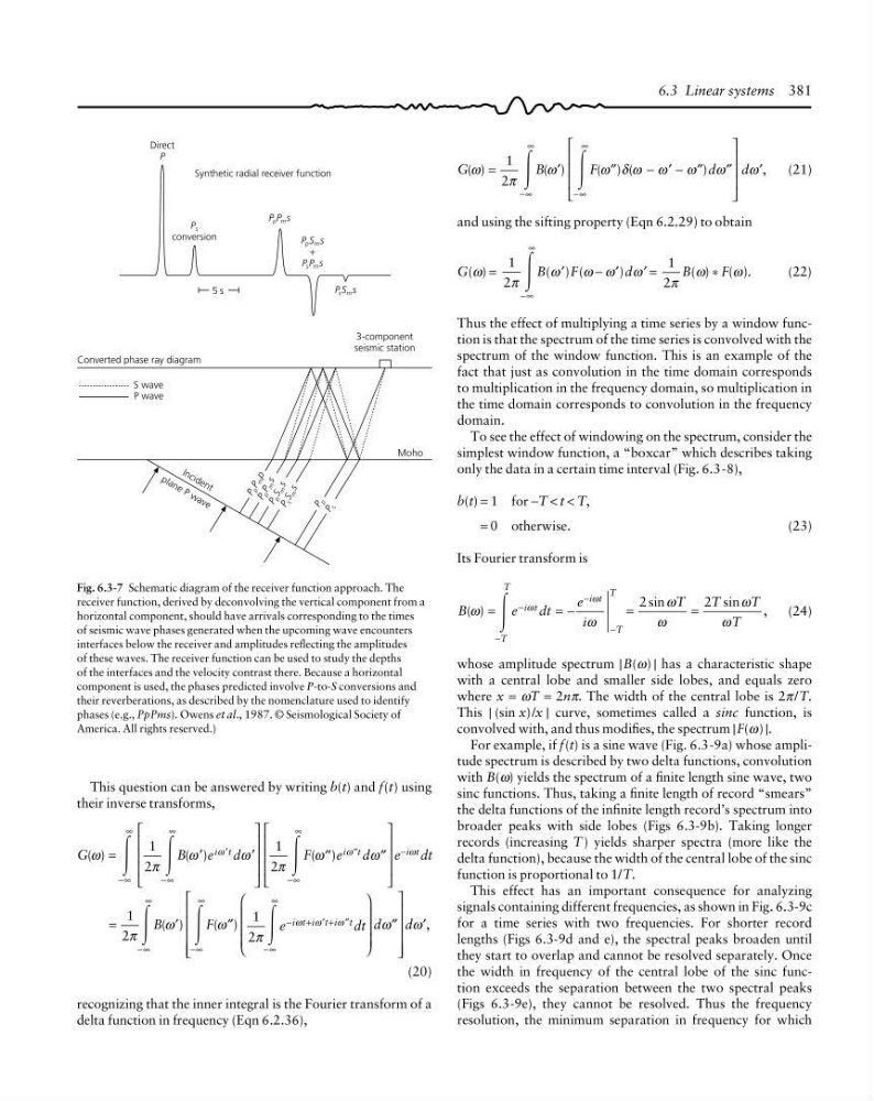
Fig. 6.3-7 Schematic diagram of the receiver function approach. The
receiver function, derived by deconvolving the vertical component from a
horizontal component, should have arrivals corresponding to the times
of seismic wave phases generated when the upcoming wave encounters
interfaces below the receiver and amplitudes reflecting the amplitudes
of these waves. The receiver function can be used to study the depths
of the interfaces and the velocity contrast there. Because a horizontal
component is used, the phases predicted involve P-to-S conversions and
their reverberations, as described by the nomenclature used to identify
phases (e.g., PpPms). Owens et al., 1987. © Seismological Society of
America. All rights reserved.)
6.3 Linear systems 381
This question can be answered by writing b(t) and f(t) using
their inverse transforms,
G
B
e d
F
e d
e d t
i t
i t
i t
( )
( )
( )
ω
π
ω
ω
π
ω
ω
ω
ω
ω
=
⎡
⎣
⎢
⎢
⎢
⎤
⎦
⎥
⎥
⎥
′′
′′
⎡
⎣
⎢
⎢
⎢
⎤
⎦
⎥
⎥
⎥
−∞
∞
−∞
∞
−∞
∞
′′
−
Ύ Ύ
Ύ
1
2
1
2
′
′
′
=
⎛
⎝
⎜
⎜
⎜
⎞
⎠
⎟
⎟
⎟
⎡
⎣
⎢
⎢
⎢
⎢
⎤
⎦
⎥
⎥
⎥
⎥
−∞
∞
−∞
∞
−∞
∞
−
+
+
( )
( )
,
1
2
1
2
π
ω
ω
π
ω
ω
ω ω
ω
Ύ Ύ
Ύ
B
F
e
d td
d
i t i t i t
′
″
″
′
′
″
(20)
recognizing that the inner integral is the Fourier transform of a
delta function in frequency (Eqn 6.2.36),
P p
P m
p
P p
P m
s
P p
S m
s
P s
S m
s
P p
P s
S wave
3-component
seismic station
Moho
p la n e P w a v e
P wave
In c id e n t
Direct
P
P s
conversion
Synthetic radial receiver function
P p P m s
P p S m s
+
P s P m s
P s S m s
5 s
G
B
F
d
d
( )
( )
( ) (
)
,
ω
π
ω
ω δω ω ω ω
ω
=
−
−
⎡
⎣
⎢
⎢
⎢
⎤
⎦
⎥
⎥
⎥
−∞
∞
−∞
∞
1
2 Ύ Ύ
′
″
′
″
″
′
(21)
and using the sifting property (Eqn 6.2.29) to obtain
G(ω) =
1
2π Ύ
−∞
∞
B(ω ′)F(ω − ω′)dω ′ =
1
2π
B(ω) * F(ω).
(22)
Thus the effect of multiplying a time series by a window function is that the spectrum of the time series is convolved with the
spectrum of the window function. This is an example of the
fact that just as convolution in the time domain corresponds
to multiplication in the frequency domain, so multiplication in
the time domain corresponds to convolution in the frequency
domain.
To see the effect of windowing on the spectrum, consider the
simplest window function, a “boxcar” which describes taking
only the data in a certain time interval (Fig. 6.3-8),
b(t) = 1 for −T < t < T,
= 0 otherwise.
(23)
Its Fourier transform is
B
e
d t
e
i
T
T
T
T
T
T
i t
i t
T
T
( )
sin
sin
,
ω
ω
ω
ω
ω
ω
ω
ω
=
=−
=
=
−
−
−
−
Ύ
2
2
(24)
whose amplitude spectrum |B(ω) | has a characteristic shape
with a central lobe and smaller side lobes, and equals zero
where x = ωT = 2nπ. The width of the central lobe is 2π /T.
This | (sin x)/x | curve, sometimes called a sinc function, is
convolved with, and thus modifies, the spectrum |F(ω) |.
For example, if f(t) is a sine wave (Fig. 6.3-9a) whose amplitude spectrum is described by two delta functions, convolution
with B(ω) yields the spectrum of a finite length sine wave, two
sinc functions. Thus, taking a finite length of record “smears”
the delta functions of the infinite length record’s spectrum into
broader peaks with side lobes (Figs 6.3-9b). Taking longer
records (increasing T ) yields sharper spectra (more like the
delta function), because the width of the central lobe of the sinc
function is proportional to 1/T.
This effect has an important consequence for analyzing
signals containing different frequencies, as shown in Fig. 6.3-9c
for a time series with two frequencies. For shorter record
lengths (Figs 6.3-9d and e), the spectral peaks broaden until
they start to overlap and cannot be resolved separately. Once
the width in frequency of the central lobe of the sinc function exceeds the separation between the two spectral peaks
(Figs 6.3-9e), they cannot be resolved. Thus the frequency
resolution, the minimum separation in frequency for which
Fig. 6.3-7 Schematic diagram of the receiver function approach. The
receiver function, derived by deconvolving the vertical component from a
horizontal component, should have arrivals corresponding to the times
of seismic wave phases generated when the upcoming wave encounters
interfaces below the receiver and amplitudes reflecting the amplitudes
of these waves. The receiver function can be used to study the depths
of the interfaces and the velocity contrast there. Because a horizontal
component is used, the phases predicted involve P-to-S conversions and
their reverberations, as described by the nomenclature used to identify
phases (e.g., PpPms). Owens et al., 1987. © Seismological Society of
America. All rights reserved.)
6.3 Linear systems 381
This question can be answered by writing b(t) and f(t) using
their inverse transforms,
G
B
e d
F
e d
e d t
i t
i t
i t
( )
( )
( )
ω
π
ω
ω
π
ω
ω
ω
ω
ω
=
⎡
⎣
⎢
⎢
⎢
⎤
⎦
⎥
⎥
⎥
′′
′′
⎡
⎣
⎢
⎢
⎢
⎤
⎦
⎥
⎥
⎥
−∞
∞
−∞
∞
−∞
∞
′′
−
Ύ Ύ
Ύ
1
2
1
2
′
′
′
=
⎛
⎝
⎜
⎜
⎜
⎞
⎠
⎟
⎟
⎟
⎡
⎣
⎢
⎢
⎢
⎢
⎤
⎦
⎥
⎥
⎥
⎥
−∞
∞
−∞
∞
−∞
∞
−
+
+
( )
( )
,
1
2
1
2
π
ω
ω
π
ω
ω
ω ω
ω
Ύ Ύ
Ύ
B
F
e
d td
d
i t i t i t
′
″
″
′
′
″
(20)
recognizing that the inner integral is the Fourier transform of a
delta function in frequency (Eqn 6.2.36),