

378 Seismograms as Signals
and regrouping terms,
y t
x f
e
d d d
i t
( )
( ) ( )
.
(
)
=
⎡
⎣
⎢
⎢
⎢
⎤
⎦
⎥
⎥
⎥
−∞
∞
−∞
∞
−∞
∞
− −
Ύ Ύ
Ύ
τ τ
π
ω τ τ
ω τ τ
′
′
′
1
2
(6)
Using the inverse transform of the delta function (Eqn 6.2.34),
1
2π
ω δ
τ τ
ω τ τ
Ύ
−∞
∞
− −
=
− −
e
d
t
i t
(
)
(
),
′
′
(7)
we eliminate the frequency integral and obtain
y t
x
f
t
d d
( )
( )
( ) (
)
.
=
− −
⎡
⎣
⎢
⎢
⎢
⎤
⎦
⎥
⎥
⎥
−∞
∞
−∞
∞
Ύ Ύ
τ
τ δ
τ τ τ τ
′
′
′
(8)
Finally, carrying out the inner integration using the sifting
property of the delta function (Eqn 6.2.29) yields
y(t) =
Ύ
−∞
∞
x(τ)f(t − τ)dτ.
(9)
This integral operation, known as the convolution of the
functions x(t) and f(t), is often written as
y(t) = x(t) * f(t).
(10)
The output of a linear system is thus the convolution of the input
signal and the impulse response. Comparison of Eqns 10 and
1 shows the relation between operations in the two domains:
convolution in the time domain corresponds to multiplication
in the frequency domain. The reverse is also true: frequency
domain convolution corresponds to time domain multiplication.
We thus have two different ways of implementing any operation that can be characterized by a linear system. The effect
that the system has on an input signal is specified either by the
impulse response in the time domain or by its transform, the
transfer function in the frequency domain. For example, to
filter a seismogram so that only a certain range of frequencies
remains, we can filter in either the frequency or time domains.
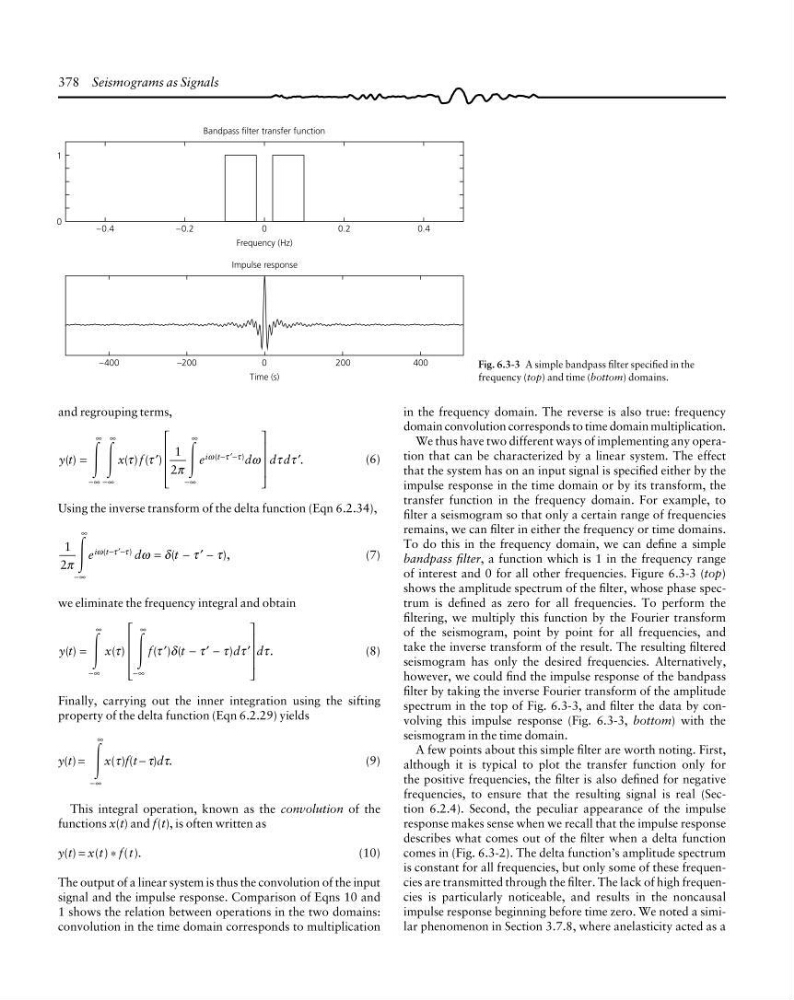
To do this in the frequency domain, we can define a simple
bandpass filter, a function which is 1 in the frequency range
of interest and 0 for all other frequencies. Figure 6.3-3 (top)
shows the amplitude spectrum of the filter, whose phase spectrum is defined as zero for all frequencies. To perform the
filtering, we multiply this function by the Fourier transform
of the seismogram, point by point for all frequencies, and
take the inverse transform of the result. The resulting filtered
seismogram has only the desired frequencies. Alternatively,
however, we could find the impulse response of the bandpass
filter by taking the inverse Fourier transform of the amplitude
spectrum in the top of Fig. 6.3-3, and filter the data by convolving this impulse response (Fig. 6.3-3, bottom) with the
seismogram in the time domain.
A few points about this simple filter are worth noting. First,
although it is typical to plot the transfer function only for
the positive frequencies, the filter is also defined for negative
frequencies, to ensure that the resulting signal is real (Section 6.2.4). Second, the peculiar appearance of the impulse
response makes sense when we recall that the impulse response
describes what comes out of the filter when a delta function
comes in (Fig. 6.3-2). The delta function’s amplitude spectrum
is constant for all frequencies, but only some of these frequencies are transmitted through the filter. The lack of high frequencies is particularly noticeable, and results in the noncausal
impulse response beginning before time zero. We noted a similar phenomenon in Section 3.7.8, where anelasticity acted as a
0.4
1
0
–0.4
–0.2
0
0.2
Frequency (Hz)
400
–400
–200
0
200
Time (s)
Impulse response
Bandpass filter transfer function
Fig. 6.3-3 A simple bandpass filter specified in the
frequency (top) and time (bottom) domains.
and regrouping terms,
y t
x f
e
d d d
i t
( )
( ) ( )
.
(
)
=
⎡
⎣
⎢
⎢
⎢
⎤
⎦
⎥
⎥
⎥
−∞
∞
−∞
∞
−∞
∞
− −
Ύ Ύ
Ύ
τ τ
π
ω τ τ
ω τ τ
′
′
′
1
2
(6)
Using the inverse transform of the delta function (Eqn 6.2.34),
1
2π
ω δ
τ τ
ω τ τ
Ύ
−∞
∞
− −
=
− −
e
d
t
i t
(
)
(
),
′
′
(7)
we eliminate the frequency integral and obtain
y t
x
f
t
d d
( )
( )
( ) (
)
.
=
− −
⎡
⎣
⎢
⎢
⎢
⎤
⎦
⎥
⎥
⎥
−∞
∞
−∞
∞
Ύ Ύ
τ
τ δ
τ τ τ τ
′
′
′
(8)
Finally, carrying out the inner integration using the sifting
property of the delta function (Eqn 6.2.29) yields
y(t) =
Ύ
−∞
∞
x(τ)f(t − τ)dτ.
(9)
This integral operation, known as the convolution of the
functions x(t) and f(t), is often written as
y(t) = x(t) * f(t).
(10)
The output of a linear system is thus the convolution of the input
signal and the impulse response. Comparison of Eqns 10 and
1 shows the relation between operations in the two domains:
convolution in the time domain corresponds to multiplication
in the frequency domain. The reverse is also true: frequency
domain convolution corresponds to time domain multiplication.
We thus have two different ways of implementing any operation that can be characterized by a linear system. The effect
that the system has on an input signal is specified either by the
impulse response in the time domain or by its transform, the
transfer function in the frequency domain. For example, to
filter a seismogram so that only a certain range of frequencies
remains, we can filter in either the frequency or time domains.
To do this in the frequency domain, we can define a simple
bandpass filter, a function which is 1 in the frequency range
of interest and 0 for all other frequencies. Figure 6.3-3 (top)
shows the amplitude spectrum of the filter, whose phase spectrum is defined as zero for all frequencies. To perform the
filtering, we multiply this function by the Fourier transform
of the seismogram, point by point for all frequencies, and
take the inverse transform of the result. The resulting filtered
seismogram has only the desired frequencies. Alternatively,
however, we could find the impulse response of the bandpass
filter by taking the inverse Fourier transform of the amplitude
spectrum in the top of Fig. 6.3-3, and filter the data by convolving this impulse response (Fig. 6.3-3, bottom) with the
seismogram in the time domain.
A few points about this simple filter are worth noting. First,
although it is typical to plot the transfer function only for
the positive frequencies, the filter is also defined for negative
frequencies, to ensure that the resulting signal is real (Section 6.2.4). Second, the peculiar appearance of the impulse
response makes sense when we recall that the impulse response
describes what comes out of the filter when a delta function
comes in (Fig. 6.3-2). The delta function’s amplitude spectrum
is constant for all frequencies, but only some of these frequencies are transmitted through the filter. The lack of high frequencies is particularly noticeable, and results in the noncausal
impulse response beginning before time zero. We noted a similar phenomenon in Section 3.7.8, where anelasticity acted as a
0.4
1
0
–0.4
–0.2
0
0.2
Frequency (Hz)
400
–400
–200
0
200
Time (s)
Impulse response
Bandpass filter transfer function
Fig. 6.3-3 A simple bandpass filter specified in the
frequency (top) and time (bottom) domains.