

Instrument
i(t)
Structure
g(t)
Source
x(t)
Seismogram
u(t)
*
*
=
f(t) * x(t);
F(ω)X(ω)
f(t)
F(ω)
x(t)
ω ω
ω
f(t) * x(t) * g(t)
F(ω)X(ω)G(ω)
g(t)
G(ω)
ω ω
ω
ω
Fig. 6.3-4 When a signal goes through two linear systems in succession,
the net output is the convolution of the impulse responses in the time
domain, or the product of the transfer functions in the frequency domain.
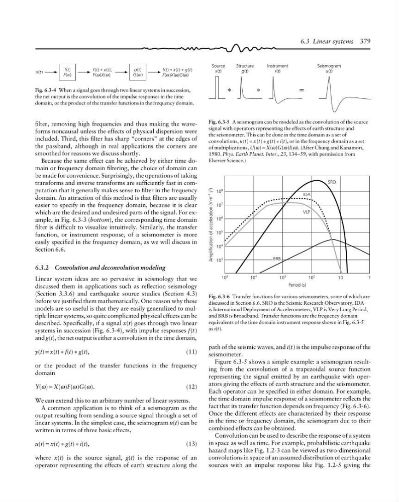
Fig. 6.3-5 A seismogram can be modeled as the convolution of the source
signal with operators representing the effects of earth structure and
the seismometer. This can be done in the time domain as a set of
convolutions, u(t) = x(t) * g(t) * i(t), or in the frequency domain as a set
of multiplications, U(ω) = X(ω)G(ω)I(ω). (After Chung and Kanamori,
1980. Phys. Earth Planet. Inter., 23, 134–59, with permission from
Elsevier Science.)
6.3 Linear systems 379
path of the seismic waves, and i(t) is the impulse response of the
seismometer.
Figure 6.3-5 shows a simple example: a seismogram resulting from the convolution of a trapezoidal source function
representing the signal emitted by an earthquake with operators giving the effects of earth structure and the seismometer.
Each operator can be specified in either domain. For example,
the time domain impulse response of a seismometer reflects the
fact that its transfer function depends on frequency (Fig. 6.3-6).
Once the different effects are characterized by their response
in the time or frequency domain, the seismogram due to their
combined effects can be obtained.
Convolution can be used to describe the response of a system
in space as well as time. For example, probabilistic earthquake
hazard maps like Fig. 1.2-3 can be viewed as two-dimensional
convolutions in space of an assumed distribution of earthquake
sources with an impulse response like Fig. 1.2-5 giving the
Amplification of acceleration (V m
–1
s
2
)
10
8
10
7
10
6
10
5
10
4
10
3
1
10
5
10
4
10
3
10
2
10
Period (s)
SRO
IDA
VLP
BRB
Fig. 6.3-6 Transfer functions for various seismometers, some of which are
discussed in Section 6.6. SRO is the Seismic Research Observatory, IDA
is International Deployment of Accelerometers, VLP is Very Long Period,
and BRB is Broadband. Transfer functions are the frequency domain
equivalents of the time domain instrument response shown in Fig. 6.3-5
as i(t).
filter, removing high frequencies and thus making the waveforms noncausal unless the effects of physical dispersion were
included. Third, this filter has sharp “corners” at the edges of
the passband, although in real applications the corners are
smoothed for reasons we discuss shortly.
Because the same effect can be achieved by either time domain or frequency domain filtering, the choice of domain can
be made for convenience. Surprisingly, the operations of taking
transforms and inverse transforms are sufficiently fast in computation that it generally makes sense to filter in the frequency
domain. An attraction of this method is that filters are usually
easier to specify in the frequency domain, because it is clear
which are the desired and undesired parts of the signal. For example, in Fig. 6.3-3 (bottom), the corresponding time domain
filter is difficult to visualize intuitively. Similarly, the transfer
function, or instrument response, of a seismometer is more
easily specified in the frequency domain, as we will discuss in
Section 6.6.
6.3.2 Convolution and deconvolution modeling
Linear system ideas are so pervasive in seismology that we
discussed them in applications such as reflection seismology
(Section 3.3.6) and earthquake source studies (Section 4.3)
before we justified them mathematically. One reason why these
models are so useful is that they are easily generalized to multiple linear systems, so quite complicated physical effects can be
described. Specifically, if a signal x(t) goes through two linear
systems in succession (Fig. 6.3-4), with impulse responses f(t)
and g(t), the net output is either a convolution in the time domain,
y(t) = x(t) * f(t) * g(t),
(11)
or the product of the transfer functions in the frequency
domain
Y(ω) = X(ω)F(ω)G(ω).
(12)
We can extend this to an arbitrary number of linear systems.
A common application is to think of a seismogram as the
output resulting from sending a source signal through a set of
linear systems. In the simplest case, the seismogram u(t) can be
written in terms of three basic effects,
u(t) = x(t) * g(t) * i(t),
(13)
where x(t) is the source signal, g(t) is the response of an
operator representing the effects of earth structure along the
i(t)
Structure
g(t)
Source
x(t)
Seismogram
u(t)
*
*
=
f(t) * x(t);
F(ω)X(ω)
f(t)
F(ω)
x(t)
ω ω
ω
f(t) * x(t) * g(t)
F(ω)X(ω)G(ω)
g(t)
G(ω)
ω ω
ω
ω
Fig. 6.3-4 When a signal goes through two linear systems in succession,
the net output is the convolution of the impulse responses in the time
domain, or the product of the transfer functions in the frequency domain.
Fig. 6.3-5 A seismogram can be modeled as the convolution of the source
signal with operators representing the effects of earth structure and
the seismometer. This can be done in the time domain as a set of
convolutions, u(t) = x(t) * g(t) * i(t), or in the frequency domain as a set
of multiplications, U(ω) = X(ω)G(ω)I(ω). (After Chung and Kanamori,
1980. Phys. Earth Planet. Inter., 23, 134–59, with permission from
Elsevier Science.)
6.3 Linear systems 379
path of the seismic waves, and i(t) is the impulse response of the
seismometer.
Figure 6.3-5 shows a simple example: a seismogram resulting from the convolution of a trapezoidal source function
representing the signal emitted by an earthquake with operators giving the effects of earth structure and the seismometer.
Each operator can be specified in either domain. For example,
the time domain impulse response of a seismometer reflects the
fact that its transfer function depends on frequency (Fig. 6.3-6).
Once the different effects are characterized by their response
in the time or frequency domain, the seismogram due to their
combined effects can be obtained.
Convolution can be used to describe the response of a system
in space as well as time. For example, probabilistic earthquake
hazard maps like Fig. 1.2-3 can be viewed as two-dimensional
convolutions in space of an assumed distribution of earthquake
sources with an impulse response like Fig. 1.2-5 giving the
Amplification of acceleration (V m
–1
s
2
)
10
8
10
7
10
6
10
5
10
4
10
3
1
10
5
10
4
10
3
10
2
10
Period (s)
SRO
IDA
VLP
BRB
Fig. 6.3-6 Transfer functions for various seismometers, some of which are
discussed in Section 6.6. SRO is the Seismic Research Observatory, IDA
is International Deployment of Accelerometers, VLP is Very Long Period,
and BRB is Broadband. Transfer functions are the frequency domain
equivalents of the time domain instrument response shown in Fig. 6.3-5
as i(t).
filter, removing high frequencies and thus making the waveforms noncausal unless the effects of physical dispersion were
included. Third, this filter has sharp “corners” at the edges of
the passband, although in real applications the corners are
smoothed for reasons we discuss shortly.
Because the same effect can be achieved by either time domain or frequency domain filtering, the choice of domain can
be made for convenience. Surprisingly, the operations of taking
transforms and inverse transforms are sufficiently fast in computation that it generally makes sense to filter in the frequency
domain. An attraction of this method is that filters are usually
easier to specify in the frequency domain, because it is clear
which are the desired and undesired parts of the signal. For example, in Fig. 6.3-3 (bottom), the corresponding time domain
filter is difficult to visualize intuitively. Similarly, the transfer
function, or instrument response, of a seismometer is more
easily specified in the frequency domain, as we will discuss in
Section 6.6.
6.3.2 Convolution and deconvolution modeling
Linear system ideas are so pervasive in seismology that we
discussed them in applications such as reflection seismology
(Section 3.3.6) and earthquake source studies (Section 4.3)
before we justified them mathematically. One reason why these
models are so useful is that they are easily generalized to multiple linear systems, so quite complicated physical effects can be
described. Specifically, if a signal x(t) goes through two linear
systems in succession (Fig. 6.3-4), with impulse responses f(t)
and g(t), the net output is either a convolution in the time domain,
y(t) = x(t) * f(t) * g(t),
(11)
or the product of the transfer functions in the frequency
domain
Y(ω) = X(ω)F(ω)G(ω).
(12)
We can extend this to an arbitrary number of linear systems.
A common application is to think of a seismogram as the
output resulting from sending a source signal through a set of
linear systems. In the simplest case, the seismogram u(t) can be
written in terms of three basic effects,
u(t) = x(t) * g(t) * i(t),
(13)
where x(t) is the source signal, g(t) is the response of an
operator representing the effects of earth structure along the