

Harmonic
e
iω 0 t
f(t) Impulse response;
F(ω) Transfer function
Linear system:
response f(t)
Impulse
δ(t)
δ
ω
y(t) = x(t) ∗ f(t);
Y(ω) = X(ω)F (ω)
Linear system:
response f(t)
Arbitrary
x(t)
ω
F(ω 0 ) e
iω0t
Linear system:
response f(t)
ω
ω ω
ω
ω
6.3 Linear systems 377
−ω 0 . If the time function were a sine rather than a cosine, the
amplitude spectrum would be the same, but the phase spectrum
would be different. Given the relation between the transforms
of functions shifted in time discussed in the previous section,
this makes sense, because a sine function is a time-shifted
cosine, and vice versa.
This example illustrates one of the reasons for using Fourier
transforms. The frequency domain description of the function
is simpler, because a large number of points are needed to
accurately describe the cosine as a function of time, but only
two complex numbers, the values of the transforms at ±ω 0 , are
needed to describe it as a function of frequency. Time series
more complicated than a pure cosine are often more easily
described in the frequency domain, and processes that act on
the time series are also often more easily represented in the
frequency domain. In such cases, it is common to work in the
frequency domain and then use the inverse transform to
generate the final time series.
6.3 Linear systems
Among the uses of Fourier analysis in seismology is modeling
different factors affecting a seismogram. First, a seismogram
is a record of ground motion that includes the effect of the
seismometer. Furthermore, the ground motion combines the
effects of the seismic source and the elastic and anelastic earth
structure along the propagation path (Section 4.3). To characterize the combined effects of these different factors, we use the
idea of a linear system, a general representation of any device
or process that takes an input signal and modifies it. This representation treats these processes as mathematical operators
transforming an input signal into an output signal.
6.3.1 Basic model
A linear system is one in which if input signals x 1 (t) and x 2 (t)
produce output signals y 1 (t) and y 2 (t), the combined input
(Ax 1 (t) + Bx 2 (t)) yields (Ay 1 (t) + By 2 (t)) (Fig. 6.3-1). We have
previously referred to this feature as the principle of superposition. Fortunately, the earth generally behaves this way in
transmitting seismic waves. As a result, linear system models
are used in a wide variety of seismological applications. Fourier
analysis is a natural tool for studying linear systems because the
Fourier transform has these same linear properties (Section 6.2.4).
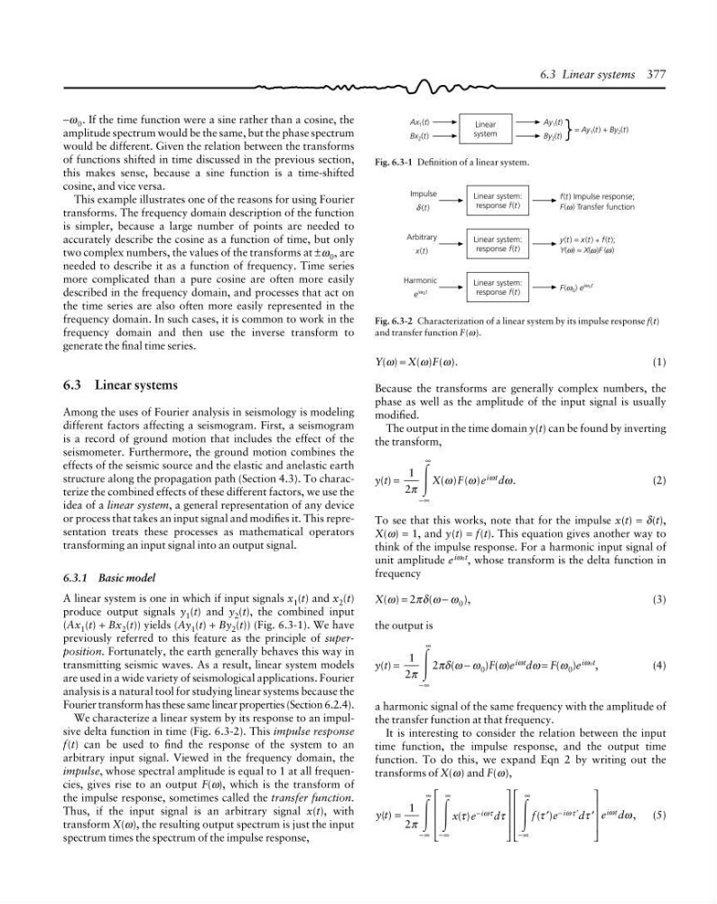
We characterize a linear system by its response to an impulsive delta function in time (Fig. 6.3-2). This impulse response
f(t) can be used to find the response of the system to an
arbitrary input signal. Viewed in the frequency domain, the
impulse, whose spectral amplitude is equal to 1 at all frequencies, gives rise to an output F(ω), which is the transform of
the impulse response, sometimes called the transfer function.
Thus, if the input signal is an arbitrary signal x(t), with
transform X(ω), the resulting output spectrum is just the input
spectrum times the spectrum of the impulse response,
Linear
system
Ax 1 (t)
Bx 2 (t)
Ay 1 (t)
By 2 (t)
= Ay 1 (t) + By 2 (t)
Fig. 6.3-1 Definition of a linear system.
Y(ω) = X(ω)F(ω).
(1)
Because the transforms are generally complex numbers, the
phase as well as the amplitude of the input signal is usually
modified.
The output in the time domain y(t) can be found by inverting
the transform,
y(t) =
1
2π Ύ
−∞
∞
X(ω)F(ω)e iωt dω.
(2)
To see that this works, note that for the impulse x(t) = δ(t),
X(ω) = 1, and y(t) = f(t). This equation gives another way to
think of the impulse response. For a harmonic input signal of
unit amplitude e
iω0t , whose transform is the delta function in
frequency
X(ω) = 2πδ(ω − ω 0 ),
(3)
the output is
y(t) =
1
2π Ύ
−∞
∞
2πδ(ω − ω 0 )F(ω)e iωt dω = F(ω 0 )e iω0t ,
(4)
a harmonic signal of the same frequency with the amplitude of
the transfer function at that frequency.
It is interesting to consider the relation between the input
time function, the impulse response, and the output time
function. To do this, we expand Eqn 2 by writing out the
transforms of X(ω) and F(ω),
y t
x e
d
f
e
d
e d
i
i
i t
( )
( )
( )
,
=
⎡
⎣
⎢
⎢
⎢
⎤
⎦
⎥
⎥
⎥
⎡
⎣
⎢
⎢
⎢
⎤
⎦
⎥
⎥
⎥
−∞
∞
−∞
∞
−
−∞
∞
−
1
2π
τ
τ
τ
τ
ω
ωτ
ω τ
ω
Ύ Ύ
Ύ ′
′
′
(5)
Fig. 6.3-2 Characterization of a linear system by its impulse response f(t)
and transfer function F(ω).
e
iω 0 t
f(t) Impulse response;
F(ω) Transfer function
Linear system:
response f(t)
Impulse
δ(t)
δ
ω
y(t) = x(t) ∗ f(t);
Y(ω) = X(ω)F (ω)
Linear system:
response f(t)
Arbitrary
x(t)
ω
F(ω 0 ) e
iω0t
Linear system:
response f(t)
ω
ω ω
ω
ω
6.3 Linear systems 377
−ω 0 . If the time function were a sine rather than a cosine, the
amplitude spectrum would be the same, but the phase spectrum
would be different. Given the relation between the transforms
of functions shifted in time discussed in the previous section,
this makes sense, because a sine function is a time-shifted
cosine, and vice versa.
This example illustrates one of the reasons for using Fourier
transforms. The frequency domain description of the function
is simpler, because a large number of points are needed to
accurately describe the cosine as a function of time, but only
two complex numbers, the values of the transforms at ±ω 0 , are
needed to describe it as a function of frequency. Time series
more complicated than a pure cosine are often more easily
described in the frequency domain, and processes that act on
the time series are also often more easily represented in the
frequency domain. In such cases, it is common to work in the
frequency domain and then use the inverse transform to
generate the final time series.
6.3 Linear systems
Among the uses of Fourier analysis in seismology is modeling
different factors affecting a seismogram. First, a seismogram
is a record of ground motion that includes the effect of the
seismometer. Furthermore, the ground motion combines the
effects of the seismic source and the elastic and anelastic earth
structure along the propagation path (Section 4.3). To characterize the combined effects of these different factors, we use the
idea of a linear system, a general representation of any device
or process that takes an input signal and modifies it. This representation treats these processes as mathematical operators
transforming an input signal into an output signal.
6.3.1 Basic model
A linear system is one in which if input signals x 1 (t) and x 2 (t)
produce output signals y 1 (t) and y 2 (t), the combined input
(Ax 1 (t) + Bx 2 (t)) yields (Ay 1 (t) + By 2 (t)) (Fig. 6.3-1). We have
previously referred to this feature as the principle of superposition. Fortunately, the earth generally behaves this way in
transmitting seismic waves. As a result, linear system models
are used in a wide variety of seismological applications. Fourier
analysis is a natural tool for studying linear systems because the
Fourier transform has these same linear properties (Section 6.2.4).
We characterize a linear system by its response to an impulsive delta function in time (Fig. 6.3-2). This impulse response
f(t) can be used to find the response of the system to an
arbitrary input signal. Viewed in the frequency domain, the
impulse, whose spectral amplitude is equal to 1 at all frequencies, gives rise to an output F(ω), which is the transform of
the impulse response, sometimes called the transfer function.
Thus, if the input signal is an arbitrary signal x(t), with
transform X(ω), the resulting output spectrum is just the input
spectrum times the spectrum of the impulse response,
Linear
system
Ax 1 (t)
Bx 2 (t)
Ay 1 (t)
By 2 (t)
= Ay 1 (t) + By 2 (t)
Fig. 6.3-1 Definition of a linear system.
Y(ω) = X(ω)F(ω).
(1)
Because the transforms are generally complex numbers, the
phase as well as the amplitude of the input signal is usually
modified.
The output in the time domain y(t) can be found by inverting
the transform,
y(t) =
1
2π Ύ
−∞
∞
X(ω)F(ω)e iωt dω.
(2)
To see that this works, note that for the impulse x(t) = δ(t),
X(ω) = 1, and y(t) = f(t). This equation gives another way to
think of the impulse response. For a harmonic input signal of
unit amplitude e
iω0t , whose transform is the delta function in
frequency
X(ω) = 2πδ(ω − ω 0 ),
(3)
the output is
y(t) =
1
2π Ύ
−∞
∞
2πδ(ω − ω 0 )F(ω)e iωt dω = F(ω 0 )e iω0t ,
(4)
a harmonic signal of the same frequency with the amplitude of
the transfer function at that frequency.
It is interesting to consider the relation between the input
time function, the impulse response, and the output time
function. To do this, we expand Eqn 2 by writing out the
transforms of X(ω) and F(ω),
y t
x e
d
f
e
d
e d
i
i
i t
( )
( )
( )
,
=
⎡
⎣
⎢
⎢
⎢
⎤
⎦
⎥
⎥
⎥
⎡
⎣
⎢
⎢
⎢
⎤
⎦
⎥
⎥
⎥
−∞
∞
−∞
∞
−
−∞
∞
−
1
2π
τ
τ
τ
τ
ω
ωτ
ω τ
ω
Ύ Ύ
Ύ ′
′
′
(5)
Fig. 6.3-2 Characterization of a linear system by its impulse response f(t)
and transfer function F(ω).