

df(t)/dt. Similarly, (iω) n F(ω) is the transform of d n f(t)/dt n .
This makes differentiation easy on a computer, and is an easy
way to change a displacement record into velocity, or velocity into acceleration. This property also makes it easy to solve
differential equations (e.g., Eqn 3.7.8) using the Fourier transform, an approach that is often posed as using a sinusoidal
trial solution. Hence we sometimes write and operate on the
wave equation using the Fourier transform of the wave field
(Eqns 2.2.34, 3.3.74).
(5) The total energy in a Fourier transform is the same as that
in the time series:
Ύ
Ύ
−∞
∞
−∞
∞
=
|
|
|
|
f t dt
F
d
( )
( )
,
2
2
1
2π
ω
ω
(27)
a relation known as Parseval’s theorem. This relation arises
because the time series and its Fourier transform are equivalent
representations.
6.2.5 Delta functions
In using Fourier transforms, we often need to describe a signal
that is concentrated at a single time or frequency. This is done
using the Dirac delta function, an entity that is not truly a function, but rather a generalized function that is the limit of a
sequence of continuous functions. The delta function can be
defined in several ways, each of which offers a different insight
into its nature.
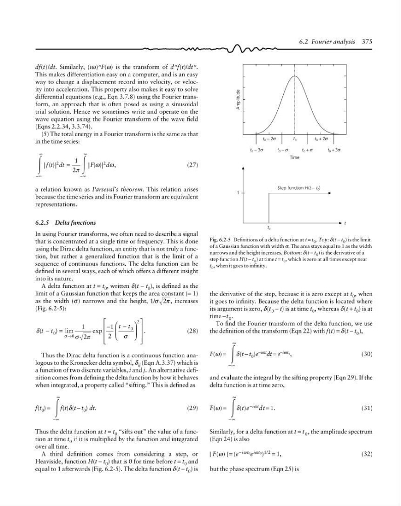
A delta function at t = t 0 , written δ(t − t 0 ), is defined as the
limit of a Gaussian function that keeps the area constant (= 1)
as the width (σ ) narrows and the height, 1
2
/σ π, increases
(Fig. 6.2-5):
δ
σ π
σ
σ
(
) lim
exp
.
t t
t t
−
=
−
−
⎛
⎝
⎜
⎞
⎠
⎟
⎡
⎣
⎢
⎢
⎢
⎤
⎦
⎥
⎥
⎥
→
0
0
0
2
1
2
1
2
(28)
Thus the Dirac delta function is a continuous function analogous to the Kronecker delta symbol, δ ij (Eqn A.3.37) which is
a function of two discrete variables, i and j. An alternative definition comes from defining the delta function by how it behaves
when integrated, a property called “sifting.” This is defined as
f(t 0 ) =
Ύ
−∞
∞
f(t)δ(t − t 0 ) dt.
(29)
Thus the delta function at t = t 0 “sifts out” the value of a function at time t 0 if it is multiplied by the function and integrated
over all time.
A third definition comes from considering a step, or
Heaviside, function H(t − t 0 ) that is 0 for time before t = t 0 and
equal to 1 afterwards (Fig. 6.2-5). The delta function δ(t − t 0 ) is
Amplitude
t 0 + 2σ
t 0
t 0 − 2σ
t 0 − 3σ
t 0 − σ
t 0 + σ
t 0 + 3σ
Time
Step function H(t − t 0 )
t 0
1
t
Fig. 6.2-5 Definitions of a delta function at t = t 0 . Top: δ(t − t 0 ) is the limit
of a Gaussian function with width σ. The area stays equal to 1 as the width
narrows and the height increases. Bottom: δ(t − t 0 ) is the derivative of a
step function H(t − t 0 ) at time t = t 0 , which is zero at all times except near
t 0 , when it goes to infinity.
the derivative of the step, because it is zero except at t 0 , when
it goes to infinity. Because the delta function is located where
its argument is zero, δ(t 0 − t) is at time t 0 , whereas δ(t + t 0 ) is at
time −t 0 .
To find the Fourier transform of the delta function, we use
the definition of the transform (Eqn 22) with f(t) = δ(t − t 0 ),
F(ω) =
Ύ
−∞
∞
δ(t − t 0 )e −iωt dt = e −iωt 0 ,
(30)
and evaluate the integral by the sifting property (Eqn 29). If the
delta function is at time zero,
F(ω) =
Ύ
−∞
∞
δ(t)e −iωt dt = 1.
(31)
Similarly, for a delta function at t = t 0 , the amplitude spectrum
(Eqn 24) is also
| F(ω) | = (e − iω t0 e iωt0 ) 1/ 2 = 1,
(32)
but the phase spectrum (Eqn 25) is
6.2 Fourier analysis 375
This makes differentiation easy on a computer, and is an easy
way to change a displacement record into velocity, or velocity into acceleration. This property also makes it easy to solve
differential equations (e.g., Eqn 3.7.8) using the Fourier transform, an approach that is often posed as using a sinusoidal
trial solution. Hence we sometimes write and operate on the
wave equation using the Fourier transform of the wave field
(Eqns 2.2.34, 3.3.74).
(5) The total energy in a Fourier transform is the same as that
in the time series:
Ύ
Ύ
−∞
∞
−∞
∞
=
|
|
|
|
f t dt
F
d
( )
( )
,
2
2
1
2π
ω
ω
(27)
a relation known as Parseval’s theorem. This relation arises
because the time series and its Fourier transform are equivalent
representations.
6.2.5 Delta functions
In using Fourier transforms, we often need to describe a signal
that is concentrated at a single time or frequency. This is done
using the Dirac delta function, an entity that is not truly a function, but rather a generalized function that is the limit of a
sequence of continuous functions. The delta function can be
defined in several ways, each of which offers a different insight
into its nature.
A delta function at t = t 0 , written δ(t − t 0 ), is defined as the
limit of a Gaussian function that keeps the area constant (= 1)
as the width (σ ) narrows and the height, 1
2
/σ π, increases
(Fig. 6.2-5):
δ
σ π
σ
σ
(
) lim
exp
.
t t
t t
−
=
−
−
⎛
⎝
⎜
⎞
⎠
⎟
⎡
⎣
⎢
⎢
⎢
⎤
⎦
⎥
⎥
⎥
→
0
0
0
2
1
2
1
2
(28)
Thus the Dirac delta function is a continuous function analogous to the Kronecker delta symbol, δ ij (Eqn A.3.37) which is
a function of two discrete variables, i and j. An alternative definition comes from defining the delta function by how it behaves
when integrated, a property called “sifting.” This is defined as
f(t 0 ) =
Ύ
−∞
∞
f(t)δ(t − t 0 ) dt.
(29)
Thus the delta function at t = t 0 “sifts out” the value of a function at time t 0 if it is multiplied by the function and integrated
over all time.
A third definition comes from considering a step, or
Heaviside, function H(t − t 0 ) that is 0 for time before t = t 0 and
equal to 1 afterwards (Fig. 6.2-5). The delta function δ(t − t 0 ) is
Amplitude
t 0 + 2σ
t 0
t 0 − 2σ
t 0 − 3σ
t 0 − σ
t 0 + σ
t 0 + 3σ
Time
Step function H(t − t 0 )
t 0
1
t
Fig. 6.2-5 Definitions of a delta function at t = t 0 . Top: δ(t − t 0 ) is the limit
of a Gaussian function with width σ. The area stays equal to 1 as the width
narrows and the height increases. Bottom: δ(t − t 0 ) is the derivative of a
step function H(t − t 0 ) at time t = t 0 , which is zero at all times except near
t 0 , when it goes to infinity.
the derivative of the step, because it is zero except at t 0 , when
it goes to infinity. Because the delta function is located where
its argument is zero, δ(t 0 − t) is at time t 0 , whereas δ(t + t 0 ) is at
time −t 0 .
To find the Fourier transform of the delta function, we use
the definition of the transform (Eqn 22) with f(t) = δ(t − t 0 ),
F(ω) =
Ύ
−∞
∞
δ(t − t 0 )e −iωt dt = e −iωt 0 ,
(30)
and evaluate the integral by the sifting property (Eqn 29). If the
delta function is at time zero,
F(ω) =
Ύ
−∞
∞
δ(t)e −iωt dt = 1.
(31)
Similarly, for a delta function at t = t 0 , the amplitude spectrum
(Eqn 24) is also
| F(ω) | = (e − iω t0 e iωt0 ) 1/ 2 = 1,
(32)
but the phase spectrum (Eqn 25) is
6.2 Fourier analysis 375