

374 Seismograms as Signals
200,000
0
400,000
Time (s)
Bolivian earthquake (M w 8.3) time series
Amplitude spectrum
600,000
0.001
0.002
Frequency (Hz)
0.003
0.004
signal as the sum of several signals, knowing that the transform
will be the sum of their transforms.
(2) The Fourier transform of a purely real time function has
the symmetry
F(−ω) = F*(ω).
(26)
Thus for seismograms (which are real because the motion of
the ground is purely real), the values of the transform for the
negative frequencies can be found from those for positive
frequencies. Hence, in filtering seismograms, we can operate on
only the positive frequencies and compute the value of the
transform at the negative frequencies by taking the conjugate,
thus saving computer time and storage space.
(3) The Fourier transform of a time series shifted in time is
found by changing the phase of the transform: if the transform
of f(t) is F(ω), the transform of f(t − a) is e −iωa F(ω). In analyzing
seismograms it is arbitrary what time we choose as the origin;
the amplitude spectrum stays the same, and the phase changes
in a simple way. This makes sense, because in the absence of
attenuation a wave keeps its shape but changes in phase as
it propagates. Similarly, shifting a Fourier transform in frequency causes a phase change in the corresponding time series:
the inverse transform of F(ω − a) is e iat f(t ). These relations are
sometimes called shift theorems.
(4) The Fourier transform of the derivative of a time function is found by multiplication: (iω)F(ω) is the transform of
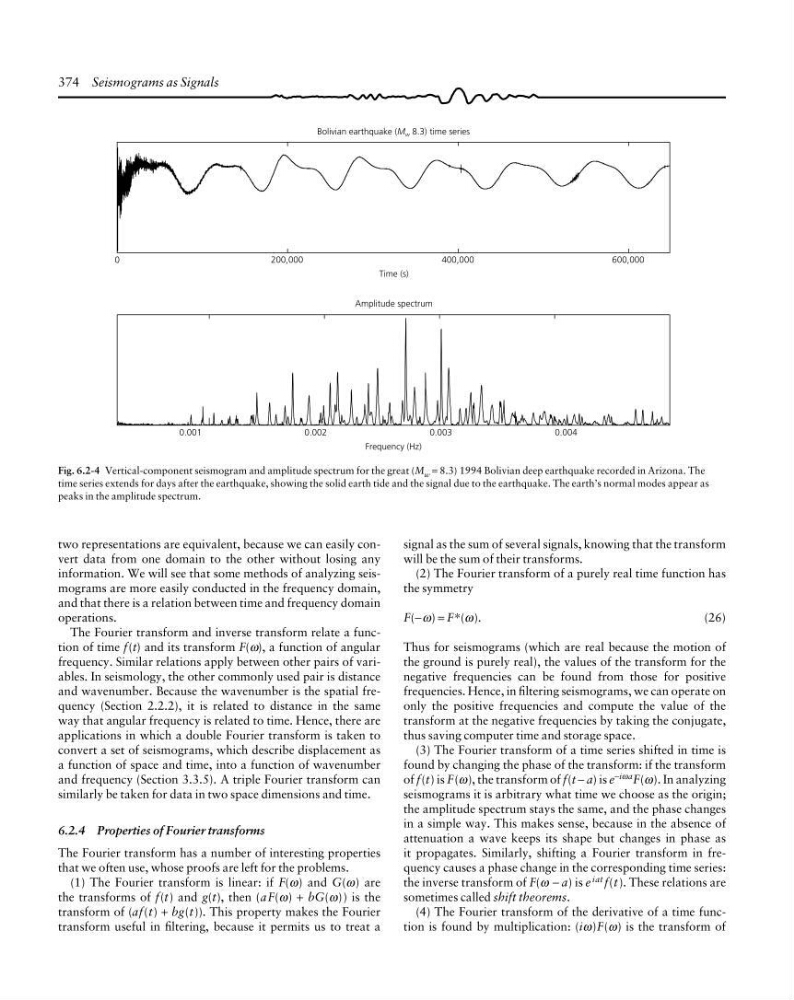
Fig. 6.2-4 Vertical-component seismogram and amplitude spectrum for the great (M w = 8.3) 1994 Bolivian deep earthquake recorded in Arizona. The
time series extends for days after the earthquake, showing the solid earth tide and the signal due to the earthquake. The earth’s normal modes appear as
peaks in the amplitude spectrum.
two representations are equivalent, because we can easily convert data from one domain to the other without losing any
information. We will see that some methods of analyzing seismograms are more easily conducted in the frequency domain,
and that there is a relation between time and frequency domain
operations.
The Fourier transform and inverse transform relate a function of time f(t) and its transform F(ω), a function of angular
frequency. Similar relations apply between other pairs of variables. In seismology, the other commonly used pair is distance
and wavenumber. Because the wavenumber is the spatial frequency (Section 2.2.2), it is related to distance in the same
way that angular frequency is related to time. Hence, there are
applications in which a double Fourier transform is taken to
convert a set of seismograms, which describe displacement as
a function of space and time, into a function of wavenumber
and frequency (Section 3.3.5). A triple Fourier transform can
similarly be taken for data in two space dimensions and time.
6.2.4 Properties of Fourier transforms
The Fourier transform has a number of interesting properties
that we often use, whose proofs are left for the problems.
(1) The Fourier transform is linear: if F(ω) and G(ω) are
the transforms of f(t) and g(t), then (aF(ω) + bG(ω)) is the
transform of (af(t) + bg(t)). This property makes the Fourier
transform useful in filtering, because it permits us to treat a
200,000
0
400,000
Time (s)
Bolivian earthquake (M w 8.3) time series
Amplitude spectrum
600,000
0.001
0.002
Frequency (Hz)
0.003
0.004
signal as the sum of several signals, knowing that the transform
will be the sum of their transforms.
(2) The Fourier transform of a purely real time function has
the symmetry
F(−ω) = F*(ω).
(26)
Thus for seismograms (which are real because the motion of
the ground is purely real), the values of the transform for the
negative frequencies can be found from those for positive
frequencies. Hence, in filtering seismograms, we can operate on
only the positive frequencies and compute the value of the
transform at the negative frequencies by taking the conjugate,
thus saving computer time and storage space.
(3) The Fourier transform of a time series shifted in time is
found by changing the phase of the transform: if the transform
of f(t) is F(ω), the transform of f(t − a) is e −iωa F(ω). In analyzing
seismograms it is arbitrary what time we choose as the origin;
the amplitude spectrum stays the same, and the phase changes
in a simple way. This makes sense, because in the absence of
attenuation a wave keeps its shape but changes in phase as
it propagates. Similarly, shifting a Fourier transform in frequency causes a phase change in the corresponding time series:
the inverse transform of F(ω − a) is e iat f(t ). These relations are
sometimes called shift theorems.
(4) The Fourier transform of the derivative of a time function is found by multiplication: (iω)F(ω) is the transform of
Fig. 6.2-4 Vertical-component seismogram and amplitude spectrum for the great (M w = 8.3) 1994 Bolivian deep earthquake recorded in Arizona. The
time series extends for days after the earthquake, showing the solid earth tide and the signal due to the earthquake. The earth’s normal modes appear as
peaks in the amplitude spectrum.
two representations are equivalent, because we can easily convert data from one domain to the other without losing any
information. We will see that some methods of analyzing seismograms are more easily conducted in the frequency domain,
and that there is a relation between time and frequency domain
operations.
The Fourier transform and inverse transform relate a function of time f(t) and its transform F(ω), a function of angular
frequency. Similar relations apply between other pairs of variables. In seismology, the other commonly used pair is distance
and wavenumber. Because the wavenumber is the spatial frequency (Section 2.2.2), it is related to distance in the same
way that angular frequency is related to time. Hence, there are
applications in which a double Fourier transform is taken to
convert a set of seismograms, which describe displacement as
a function of space and time, into a function of wavenumber
and frequency (Section 3.3.5). A triple Fourier transform can
similarly be taken for data in two space dimensions and time.
6.2.4 Properties of Fourier transforms
The Fourier transform has a number of interesting properties
that we often use, whose proofs are left for the problems.
(1) The Fourier transform is linear: if F(ω) and G(ω) are
the transforms of f(t) and g(t), then (aF(ω) + bG(ω)) is the
transform of (af(t) + bg(t)). This property makes the Fourier
transform useful in filtering, because it permits us to treat a