

372 Seismograms as Signals
∆ω = (2π /T )∆n
(18)
so that
∆n = (T∆ω)/(2π)
(19)
and
f t
F T
e
n
n
i t
n
( )
( / )
.
=
=−∞
∞
∑
2π
ω
ω
∆
(20)
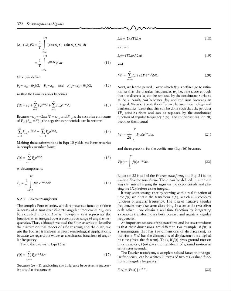
Next, we let the period T over which f(t) is defined go to infinity, so that the angular frequencies ω n become close enough
that the discrete ω n can be replaced by the continuous variable
ω. As a result, ∆ω becomes dω, and the sum becomes an
integral. We assert (note the difference between seismology and
mathematics texts) that this can be done such that the product
TF n remains finite and can be replaced by the continuous
function of angular frequency F(ω). The Fourier series (Eqn 20)
becomes the integral
f t
F e d
i t
( )
( )
,
=
−∞
∞
1
2π
ω
ω
ω
Ύ
(21)
and the expression for the coefficients (Eqn 16) becomes
F
fte
d t
i t
( )
( )
.
ω
ω
=
−∞
∞
−
Ύ
(22)
Equation 22 is called the Fourier transform, and Eqn 21 is the
inverse Fourier transform. These can be defined in alternate
ways by interchanging the signs on the exponentials and placing the 1/2π before either integral.
It may seem strange that by starting with a real function of
time f(t) we obtain the transform F(ω), which is a complex
function of angular frequency. The idea of negative angular
frequencies may also seem disturbing. In a sense the two offset
each other a we obtain a real time function by integrating
a complex transform over both positive and negative angular
frequencies.
An important feature of the transform and inverse transform
is that their dimensions are different. For example, if f(t) is
a seismogram that has the dimensions of displacement, its
transform F(ω) has the dimensions of displacement multiplied
by time (from the dt term). Thus, if f(t) gives ground motion
in centimeters, F(ω) gives the transform of ground motion in
centimeter-seconds.
The Fourier transform, a complex-valued function of angular frequency, can be written in terms of two real-valued functions of angular frequency:
F(ω) = | F(ω) | e iφ(ω) ,
(23)
(
)/
[cos
sin
] ( )
/
/
a
ib
T
t i
t f t dt
n
n
T
T
n
n
+
=
+
−
2
1
2
2
Ύ
ω
ω
=
−
( ) .
/
/
1
2
2
T
e f t dt
T
T
i t
n
Ύ
ω
(11)
Next, we define
F n = (a n − ib n )/2, F 0 = a 0 , and F −n = (a n + ib n )/2,
(12)
so that the Fourier series becomes
f t F
F e
F e
n
n
i t
n
n
i t
n
n
( )
.
=
+
+
=
∞
=
∞
−
−
∑
∑
0
1
1
ω
ω
(13)
Because −ω n = −2nπ /T = ω − n and F −n is the complex conjugate
of F n , (F −n = F* n ), the negative exponentials can be written
n
n
i t
n
n
i t
F e
F e
n
n
=
∞
−
−
= −
−∞
∑
∑
=
1
1
ω
ω .
(14)
Making these substitutions in Eqn 10 yields the Fourier series
in complex number form:
f t
F e
n
n
i t
n
( )
,
=
=−∞
∞
∑
ω
(15)
with components
F
T
f t e
dt
n
T
T
i t
n
( )
.
/
/
=
−
−
1
2
2
Ύ
ω
(16)
6.2.3 Fourier transforms
The complex Fourier series, which represents a function of time
in terms of a sum over discrete angular frequencies ω n , can
be extended into the Fourier transform that represents the
function as an integral over a continuous range of angular frequencies. Thus, although we used the Fourier series to describe
the discrete normal modes of a finite string and the earth, we
use the Fourier transform in most seismological applications,
because we regard the waves as continuous functions of angular frequency.
To do this, we write Eqn 15 as
f t
F e
n
n
n
i t
n
( ) =
=−∞
∞
∑
ω
∆
(17)
(because ∆n = 1), and define the difference between the successive angular frequencies
∆ω = (2π /T )∆n
(18)
so that
∆n = (T∆ω)/(2π)
(19)
and
f t
F T
e
n
n
i t
n
( )
( / )
.
=
=−∞
∞
∑
2π
ω
ω
∆
(20)
Next, we let the period T over which f(t) is defined go to infinity, so that the angular frequencies ω n become close enough
that the discrete ω n can be replaced by the continuous variable
ω. As a result, ∆ω becomes dω, and the sum becomes an
integral. We assert (note the difference between seismology and
mathematics texts) that this can be done such that the product
TF n remains finite and can be replaced by the continuous
function of angular frequency F(ω). The Fourier series (Eqn 20)
becomes the integral
f t
F e d
i t
( )
( )
,
=
−∞
∞
1
2π
ω
ω
ω
Ύ
(21)
and the expression for the coefficients (Eqn 16) becomes
F
fte
d t
i t
( )
( )
.
ω
ω
=
−∞
∞
−
Ύ
(22)
Equation 22 is called the Fourier transform, and Eqn 21 is the
inverse Fourier transform. These can be defined in alternate
ways by interchanging the signs on the exponentials and placing the 1/2π before either integral.
It may seem strange that by starting with a real function of
time f(t) we obtain the transform F(ω), which is a complex
function of angular frequency. The idea of negative angular
frequencies may also seem disturbing. In a sense the two offset
each other a we obtain a real time function by integrating
a complex transform over both positive and negative angular
frequencies.
An important feature of the transform and inverse transform
is that their dimensions are different. For example, if f(t) is
a seismogram that has the dimensions of displacement, its
transform F(ω) has the dimensions of displacement multiplied
by time (from the dt term). Thus, if f(t) gives ground motion
in centimeters, F(ω) gives the transform of ground motion in
centimeter-seconds.
The Fourier transform, a complex-valued function of angular frequency, can be written in terms of two real-valued functions of angular frequency:
F(ω) = | F(ω) | e iφ(ω) ,
(23)
(
)/
[cos
sin
] ( )
/
/
a
ib
T
t i
t f t dt
n
n
T
T
n
n
+
=
+
−
2
1
2
2
Ύ
ω
ω
=
−
( ) .
/
/
1
2
2
T
e f t dt
T
T
i t
n
Ύ
ω
(11)
Next, we define
F n = (a n − ib n )/2, F 0 = a 0 , and F −n = (a n + ib n )/2,
(12)
so that the Fourier series becomes
f t F
F e
F e
n
n
i t
n
n
i t
n
n
( )
.
=
+
+
=
∞
=
∞
−
−
∑
∑
0
1
1
ω
ω
(13)
Because −ω n = −2nπ /T = ω − n and F −n is the complex conjugate
of F n , (F −n = F* n ), the negative exponentials can be written
n
n
i t
n
n
i t
F e
F e
n
n
=
∞
−
−
= −
−∞
∑
∑
=
1
1
ω
ω .
(14)
Making these substitutions in Eqn 10 yields the Fourier series
in complex number form:
f t
F e
n
n
i t
n
( )
,
=
=−∞
∞
∑
ω
(15)
with components
F
T
f t e
dt
n
T
T
i t
n
( )
.
/
/
=
−
−
1
2
2
Ύ
ω
(16)
6.2.3 Fourier transforms
The complex Fourier series, which represents a function of time
in terms of a sum over discrete angular frequencies ω n , can
be extended into the Fourier transform that represents the
function as an integral over a continuous range of angular frequencies. Thus, although we used the Fourier series to describe
the discrete normal modes of a finite string and the earth, we
use the Fourier transform in most seismological applications,
because we regard the waves as continuous functions of angular frequency.
To do this, we write Eqn 15 as
f t
F e
n
n
n
i t
n
( ) =
=−∞
∞
∑
ω
∆
(17)
(because ∆n = 1), and define the difference between the successive angular frequencies